Estimating the Fisher Hypothesis Using Linear Regression
In this tutorial, we utilise the R programming language for linear regression modelling as well as for conducting hypothesis tests and inferential statistical analysis for significance of coefficients and testing normality of residuals.
With this example, you will Learn to use R programming for
- Estimating a linear regression model
- Finding slope coefficients and intercept coefficients of a linear regression model using R
- Testing the significance of slope coefficient of a linear regression model using R
- Constructing a residual plot for linear regression model in R
The data used in this exercise is the United States quarterly data for the period 1954: Q3 to 2007: Q4 on the nominal interest rate, rt, the price level, pt, and inflation, πt.
The Fisher hypothesis states that nominal interest rates, r, fully reflect long-run movements in expected inflation, E(π), or
r = i + E(π)
where i is the real interest rate
If the real interest rate is assumed to be constant, then there will be a one-for-one adjustment of the nominal interest rate to the expected inflation rate.
To test this model in a linear regression setting consider model rt = β0 + β1 E(πt) + ut, where ut is a disturbance term.
The expected rate of inflation is unobservable and so the model as it stands cannot be estimated.
On the assumption that expectations are formed in a rational way so that, on average, expected inflation is equal to realised inflation, gives πt = E(πt) + wt where wt is the zero-mean error in the expectation.
A test of the Fisher hypothesis can be formulated as a test of β1 = 1 in the linear regression model rt = β0 + β1πt + et, in which et is now the composite error term ut − wt.
The statistical analysis is done using R. Click here to know more about R software for statistics.
Step1: Downloading the USA Inflation (CPI) and Nominal Interest Rates (Fed Funds) data
Learn how to load data sets in R
Table 1: Inflation (CPI) and Nominal Interest rates (Fed Funds) in USA
| DATE | CPI | FED FUNDS |
|---|---|---|
| 1956-01-01 | 0.374532 | 2.48 |
| 1956-04-01 | 1.248439 | 2.69 |
| 1956-07-01 | 1.987578 | 2.81 |
| 1956-10-01 | 2.48139 | 2.93 |
| 1957-01-01 | 3.358209 | 2.93 |
| 1957-04-01 | 3.575832 | 3.00 |
| 1957-07-01 | 3.410475 | 3.23 |
| 1957-10-01 | 3.026634 | 3.25 |
| 1958-01-01 | 3.489771 | 1.86 |
| 1958-04-01 | 3.214286 | 0.94 |
| 1958-07-01 | 2.237927 | 1.32 |
| 1958-10-01 | 1.99765 | 2.16 |
More table records
| DATE | CPI | FED FUNDS |
|---|---|---|
| 1959-01-01 | 0.930233 | 2.57 |
| 1959-04-01 | 0.461361 | 3.08 |
| 1959-07-01 | 1.036866 | 3.58 |
| 1959-10-01 | 1.612903 | 3.99 |
| 1960-01-01 | 1.497696 | 3.93 |
| 1960-04-01 | 1.722158 | 3.70 |
| 1960-07-01 | 1.254276 | 2.94 |
| 1960-10-01 | 1.360544 | 2.30 |
| 1961-01-01 | 1.475596 | 2.00 |
| 1961-04-01 | 0.902935 | 1.73 |
| 1961-07-01 | 1.238739 | 1.68 |
| 1961-10-01 | 0.671141 | 2.40 |
| 1962-01-01 | 0.894855 | 2.46 |
| 1962-04-01 | 1.342282 | 2.61 |
| 1962-07-01 | 1.223582 | 2.85 |
| 1962-10-01 | 1.333333 | 2.92 |
| 1963-01-01 | 1.219512 | 2.97 |
| 1963-04-01 | 1.103753 | 2.96 |
| 1963-07-01 | 1.208791 | 3.33 |
| 1963-10-01 | 1.425439 | 3.45 |
| 1964-01-01 | 1.533406 | 3.46 |
| 1964-04-01 | 1.310044 | 3.49 |
| 1964-07-01 | 1.194354 | 3.46 |
| 1964-10-01 | 1.081081 | 3.58 |
| 1965-01-01 | 1.078749 | 3.97 |
| 1965-04-01 | 1.724138 | 4.08 |
| 1965-07-01 | 1.716738 | 4.07 |
| 1965-10-01 | 1.818182 | 4.17 |
| 1966-01-01 | 2.347919 | 4.56 |
| 1966-04-01 | 2.754237 | 4.91 |
| 1966-07-01 | 3.270042 | 5.41 |
| 1966-10-01 | 3.676471 | 5.56 |
| 1967-01-01 | 3.023983 | 4.82 |
| 1967-04-01 | 2.680412 | 3.99 |
| 1967-07-01 | 2.655771 | 3.89 |
| 1967-10-01 | 2.735562 | 4.17 |
| 1968-01-01 | 3.846154 | 4.79 |
| 1968-04-01 | 4.016064 | 5.98 |
| 1968-07-01 | 4.477612 | 5.94 |
| 1968-10-01 | 4.733728 | 5.92 |
| 1969-01-01 | 4.775828 | 6.57 |
| 1969-04-01 | 5.501931 | 8.33 |
| 1969-07-01 | 5.619048 | 8.98 |
| 1969-10-01 | 5.932203 | 8.94 |
| 1970-01-01 | 6.046512 | 8.57 |
| 1970-04-01 | 6.038426 | 7.88 |
| 1970-07-01 | 5.680793 | 6.70 |
| 1970-10-01 | 5.6 | 5.57 |
| 1971-01-01 | 5 | 3.86 |
| 1971-04-01 | 4.400345 | 4.56 |
| 1971-07-01 | 4.351536 | 5.47 |
| 1971-10-01 | 3.451179 | 4.75 |
| 1972-01-01 | 3.42523 | 3.54 |
| 1972-04-01 | 3.140496 | 4.30 |
| 1972-07-01 | 3.025347 | 4.74 |
| 1972-10-01 | 3.49878 | 5.14 |
| 1973-01-01 | 4.038772 | 6.54 |
| 1973-04-01 | 5.528846 | 7.82 |
| 1973-07-01 | 6.825397 | 10.56 |
| 1973-10-01 | 8.254717 | 10.00 |
| 1974-01-01 | 9.937888 | 9.32 |
| 1974-04-01 | 10.55429 | 11.25 |
| 1974-07-01 | 11.44131 | 12.09 |
| 1974-10-01 | 12.20044 | 9.35 |
| 1975-01-01 | 11.08757 | 6.30 |
| 1975-04-01 | 9.684066 | 5.42 |
| 1975-07-01 | 8.733334 | 6.16 |
| 1975-10-01 | 7.249191 | 5.41 |
| 1976-01-01 | 6.357279 | 4.83 |
| 1976-04-01 | 6.073889 | 5.20 |
| 1976-07-01 | 5.518087 | 5.28 |
| 1976-10-01 | 5.069403 | 4.87 |
| 1977-01-01 | 5.85774 | 4.66 |
| 1977-04-01 | 6.847698 | 5.16 |
| 1977-07-01 | 6.682161 | 5.82 |
| 1977-10-01 | 6.605399 | 6.51 |
| 1978-01-01 | 6.606437 | 6.76 |
| 1978-04-01 | 6.961326 | 7.28 |
| 1978-07-01 | 7.95207 | 8.10 |
| 1978-10-01 | 8.943966 | 9.58 |
| 1979-01-01 | 9.745763 | 10.07 |
| 1979-04-01 | 10.7438 | 10.18 |
| 1979-07-01 | 11.7558 | 10.95 |
| 1979-10-01 | 12.66073 | 13.58 |
| 1980-01-01 | 14.28571 | 15.05 |
| 1980-04-01 | 14.5056 | 12.69 |
| 1980-07-01 | 12.86682 | 9.84 |
| 1980-10-01 | 12.64267 | 15.85 |
| 1981-01-01 | 11.23311 | 16.57 |
| 1981-04-01 | 9.775968 | 17.78 |
| 1981-07-01 | 10.84 | 17.58 |
| 1981-10-01 | 9.547935 | 13.59 |
| 1982-01-01 | 7.593014 | 14.23 |
| 1982-04-01 | 6.753247 | 14.51 |
| 1982-07-01 | 5.774089 | 11.01 |
| 1982-10-01 | 4.517965 | 9.29 |
| 1983-01-01 | 3.599153 | 8.65 |
| 1983-04-01 | 3.336809 | 8.80 |
| 1983-07-01 | 2.62709 | 9.46 |
| 1983-10-01 | 3.301566 | 9.43 |
| 1984-01-01 | 4.529973 | 9.69 |
| 1984-04-01 | 4.339051 | 10.56 |
| 1984-07-01 | 4.255319 | 11.39 |
| 1984-10-01 | 4.085667 | 9.27 |
| 1985-01-01 | 3.584229 | 8.48 |
| 1985-04-01 | 3.739523 | 7.92 |
| 1985-07-01 | 3.348214 | 7.90 |
| 1985-10-01 | 3.51377 | 8.10 |
| 1986-01-01 | 3.082731 | 7.83 |
| 1986-04-01 | 1.615911 | 6.92 |
| 1986-07-01 | 1.635298 | 6.21 |
| 1986-10-01 | 1.284404 | 6.27 |
| 1987-01-01 | 2.197132 | 6.22 |
| 1987-04-01 | 3.761468 | 6.65 |
| 1987-07-01 | 4.189435 | 6.84 |
| 1987-10-01 | 4.498792 | 6.92 |
| 1988-01-01 | 3.971335 | 6.66 |
| 1988-04-01 | 3.919835 | 7.16 |
| 1988-07-01 | 4.108392 | 7.98 |
| 1988-10-01 | 4.305114 | 8.47 |
| 1989-01-01 | 4.824813 | 9.44 |
| 1989-04-01 | 5.218378 | 9.73 |
| 1989-07-01 | 4.673944 | 9.08 |
| 1989-10-01 | 4.598338 | 8.61 |
| 1990-01-01 | 5.232877 | 8.25 |
| 1990-04-01 | 4.58221 | 8.24 |
| 1990-07-01 | 5.53476 | 8.16 |
| 1990-10-01 | 6.223517 | 7.74 |
| 1991-01-01 | 5.285082 | 6.43 |
| 1991-04-01 | 4.845361 | 5.86 |
| 1991-07-01 | 3.876362 | 5.64 |
| 1991-10-01 | 2.991773 | 4.82 |
| 1991-10-01 | 2.991773 | 4.82 |
| 1992-01-01 | 2.868447 | 4.02 |
| 1992-04-01 | 3.097345 | 3.77 |
| 1992-07-01 | 3.097561 | 3.26 |
| 1992-10-01 | 3.050109 | 3.04 |
| 1993-01-01 | 3.197115 | 3.04 |
| 1993-04-01 | 3.147353 | 3.00 |
| 1993-07-01 | 2.744263 | 3.06 |
| 1993-10-01 | 2.724924 | 2.99 |
| 1994-01-01 | 2.515723 | 3.21 |
| 1994-04-01 | 2.380952 | 3.94 |
| 1994-07-01 | 2.878195 | 4.49 |
| 1994-10-01 | 2.652641 | 5.17 |
| 1995-01-01 | 2.840264 | 5.81 |
| 1995-04-01 | 3.093249 | 6.02 |
| 1995-07-01 | 2.641003 | 5.80 |
| 1995-10-01 | 2.650924 | 5.72 |
| 1996-01-01 | 2.739726 | 5.36 |
| 1996-04-01 | 2.847131 | 5.24 |
| 1996-07-01 | 2.943742 | 5.31 |
| 1996-10-01 | 3.190104 | 5.28 |
| 1997-01-01 | 2.946237 | 5.28 |
| 1997-04-01 | 2.342419 | 5.52 |
| 1997-07-01 | 2.202923 | 5.53 |
| 1997-10-01 | 1.871714 | 5.51 |
| 1998-01-01 | 1.462294 | 5.52 |
| 1998-04-01 | 1.602164 | 5.50 |
| 1998-07-01 | 1.595855 | 5.53 |
| 1998-10-01 | 1.548307 | 4.86 |
| 1999-01-01 | 1.667696 | 4.73 |
| 1999-04-01 | 2.109359 | 4.75 |
| 1999-07-01 | 2.345981 | 5.09 |
| 1999-10-01 | 2.622484 | 5.31 |
| 2000-01-01 | 3.240178 | 5.68 |
| 2000-04-01 | 3.329322 | 6.27 |
| 2000-07-01 | 3.508073 | 6.52 |
| 2000-10-01 | 3.4271 | 6.47 |
| 2001-01-01 | 3.393488 | 5.59 |
| 2001-04-01 | 3.377329 | 4.33 |
| 2001-07-01 | 2.695937 | 3.50 |
| 2001-10-01 | 1.857882 | 2.13 |
| 2002-01-01 | 1.252134 | 1.73 |
| 2002-04-01 | 1.295531 | 1.75 |
| 2002-07-01 | 1.59385 | 1.74 |
| 2002-10-01 | 2.200075 | 1.44 |
| 2003-01-01 | 2.866779 | 1.25 |
| 2003-04-01 | 2.131603 | 1.25 |
| 2003-07-01 | 2.196383 | 1.02 |
| 2003-10-01 | 1.895124 | 1.00 |
| 2004-01-01 | 1.785064 | 1.00 |
| 2004-04-01 | 2.867514 | 1.01 |
| 2004-07-01 | 2.727108 | 1.43 |
| 2004-10-01 | 3.322499 | 1.95 |
| 2005-01-01 | 3.042233 | 2.47 |
| 2005-04-01 | 2.946366 | 2.94 |
| 2005-07-01 | 3.83263 | 3.46 |
| 2005-10-01 | 3.739951 | 3.98 |
| 2006-01-01 | 3.6471 | 4.46 |
| 2006-04-01 | 4.010283 | 4.91 |
| 2006-07-01 | 3.335591 | 5.25 |
| 2006-10-01 | 1.937332 | 5.25 |
| 2007-01-01 | 2.424095 | 5.26 |
| 2007-04-01 | 2.650684 | 5.25 |
| 2007-07-01 | 2.360478 | 5.07 |
| 2007-10-01 | 3.974384 | 4.50 |
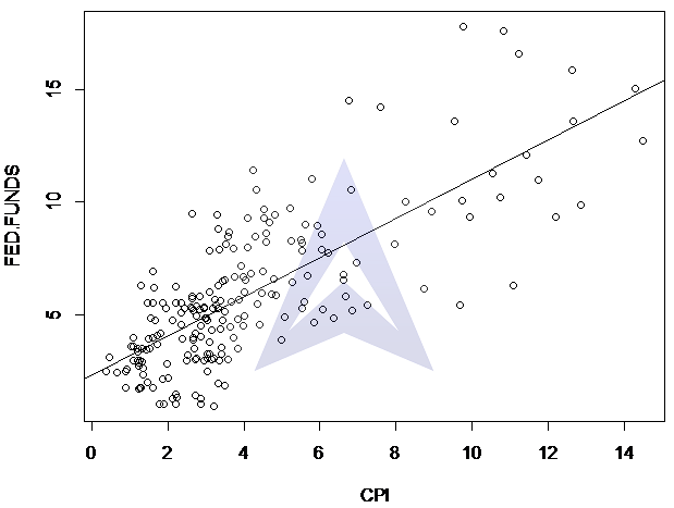
Step 2: Draw a scatter plot of rt and πt and superimpose a line of best fit in order to get a visual appreciation of the relationship between nominal interest rates and actual inflation.
The following scatter plot and line of best fit shows the relationship between nominal interest rates (Fed funds) and actual inflation (CPI):

Step 3: Estimate the linear regression version of the Fisher equation and interpret the parameter estimates.
We have carried out the estimation of Fisher model using linear regression function in R software. To test the Fisher hypothesis model in a linear regression setting consider the model
{`
rt = β0 + β1 E(πt) + ut
where ut is a disturbance term.
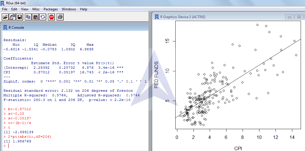
The result of regression (obtained from R) are as follows:
`}
{`
lm(formula = FED.FUNDS ~ CPI, data = fisher)

Residuals:
Min        1Q  	    Median    3Q       Max
-5.6314    -1.5541  -0.0783   1.0902   6.9898

Coefficients:
Estimate     Std. Error   t value   Pr(>|t|)
(Intercept) 	2.28392      0.25732      8.876     3.4e-16 ***
CPI        	0.87012      0.05197 	  16.743    < 2e-16 ***
---
Signif. codes:  0 ‘***’ 0.001 ‘**’ 0.01 ‘*’ 0.05 ‘.’ 0.1 ‘ ’ 1
`}
Residual standard error: 2.132 on 206 degrees of freedom
Multiple R-squared: 0.5764, Adjusted R-squared: 0.5744
F-statistic: 280.3 on 1 and 206 DF, p-value:
< 2.2e-16
The model Fisher equation is rt = β0 + β1*πt + et
where rt = nominal interest rate
πt = inflation rate
and et is the composite error term = ut – wt
The actual estimated coefficient of β0 and β1 is
FEDFUND = 2.28392 + 0.87012 (CPI)
This means that with a 1% change in inflation (CPI), nominal interest rate (FEDFUND) increases by 0.87012%.
The fixed component of the nominal interest rate is 2.23892 and the R-square value of the estimated model implies that 57.44% of the change in nominal interest rate is explained by change in inflation.
Learn more about linear regression using R
Step 4: Testing for Restrictions and significance of Slope Coefficient
Test the restriction β1 = 1 for the estimated Fisher Model and interpret the result. In particular, interpret the estimate of β0 when β1 = 1.
Consider
Null hypothesis: H0: β1 = 1
Alternate hypothesis: H1: β1≠1
We will use the t test to test this restriction based on the following specifications:
{`
Estimated β1= 0.87012
Level of significance, α= 0.05
Standard error, S.E.= 0.05197
`}
Then the t-statistic is calculated as follows:
tcal=(β1-1)/(standard error)= -2.499
|tcal |= 2.499
The Critical t value for this case with based on degree of freedom and level of significance is 1.987. The t-statistic can also be calculated in R program as shown below:

Since |tcal |> critical value, we reject the null hypothesis H0.
Thus, it can be concluded that there is sufficient evidence to believe that β1 ≠ 1. Thus, the slope is 0.87012. Therefore, Fishers equation is not satisfied.
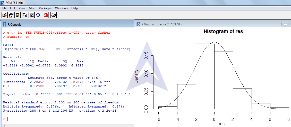
Whenβ1 = 1, the intercept estimate (β0 ) remains the same as earlier. This shows that the intercept value is independent of the slope. The regression results when β1 =1 are as follows:

Step 5: Plotting the residuals from Linear Regression Model in R
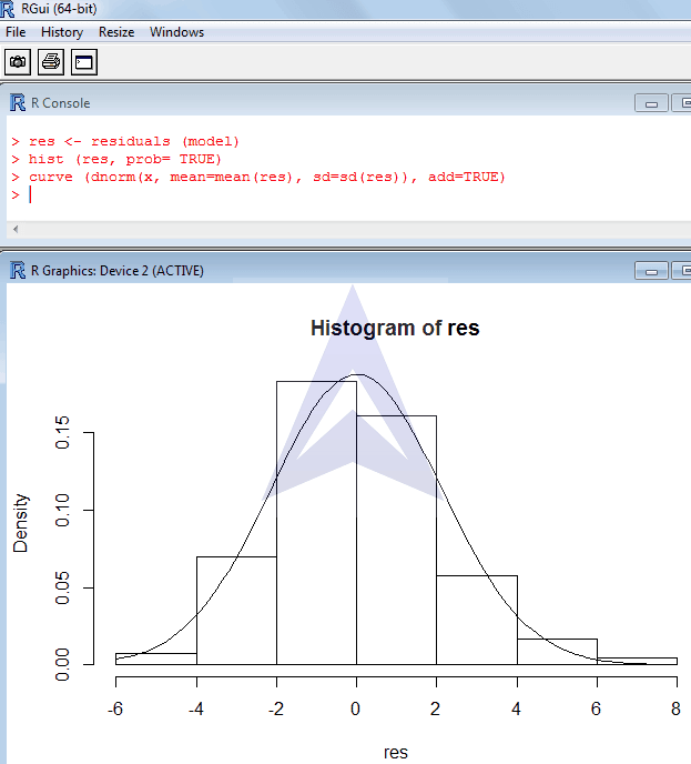
Draw a histogram of the residuals with a normal distribution overlaid on it.
The histogram of residuals with a normal distribution overlaid on it is given below (along with the R commands):

Looking for more help with R programming for statistical analysis and econometrics? Learn and master R for statistics, data science, data analysis, econometrics and business management using this free R tutorial created by Assignmenthelp.net online statistics tutors.


