Monthly Data Time Series Analysis: De-Trending
The following data (stored in Credit) are monthly credit card charges (in millions of dollars) for a popular credit card issued by a large bank (the mane of which is not disclosed at its request):
| Month | 2007 | 2008 | 2009 |
|---|---|---|---|
| January | 31.9 | 39.4 | 45.0 |
| February | 27.0 | 36.2 | 39.6 |
| March | 31.3 | 40.5 | |
| April | 39.4 | 46.8 | |
| May | 39.4 | 46.8 | |
| June | 40.7 | 44.7 | |
| July | 42.3 | 52.2 | |
| August | 49.5 | 54.0 | |
| September | 45.0 | 48.8 | |
| October | 50.0 | 55.8 | |
| November | 50.9 | 58.7 | |
| December | 58.5 | 63.4 |
A. Construct the time-series plot
Copy the data and paste it into the Excel sheet.
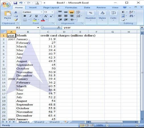
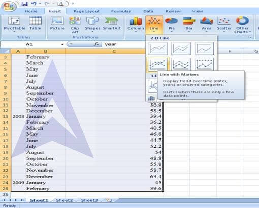
To construct the time series plot, select the data and go to Insert -> Line -> Line with marker.
The following time series plot will be created.
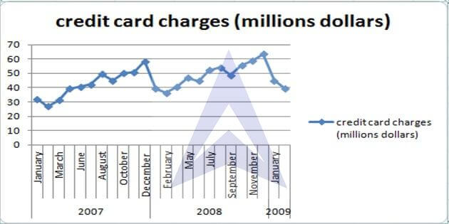
B. Describe the monthly pattern that is evident in the data
From the data, it can be observed that the credit card charges exhibit a rising trend over a one-year cycle. In the starting of the year the charges decline continuously in the month of January and February, reaching their lowest-in-the-year value in the month of February. After February, the charges pick up and continue to rise but dip once in September every year. In the month of December, the charges are highest.
C. In general, would you say that the overall dollar amounts charged on the bank’s credit cards is increasing or decreasing? Explain
It can be observed that the overall charges are increasing every year, i.e., the charges in January 2009 are higher than those in January 2008, which in turn is higher than that in January 2007. Similar observation is made for all the months. Thus the data is depicting an upward sloping trend line overall, despite monthly fluctuations.
D. Note that December 2008 charges were more than $63 million, but those for February 2009 were less than $40 million. Was February’s total close to what you would have expected?
Step 1: Select the data and go to Insert -> Pivot Table
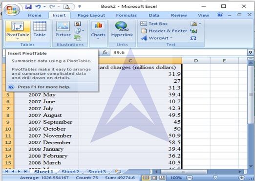
Step 2: In the Pivot Table dialog box, select the data range as A1 to C25.
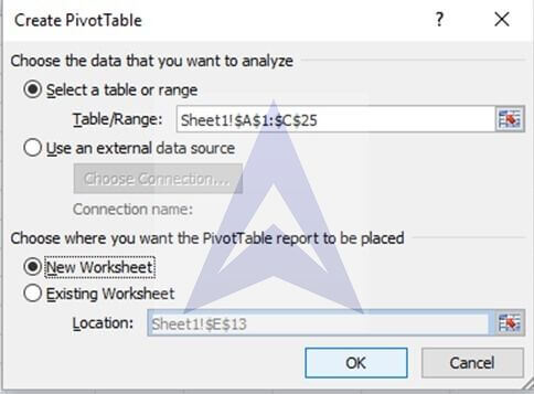
Step 3: On clicking on Ok, the following screen appears:
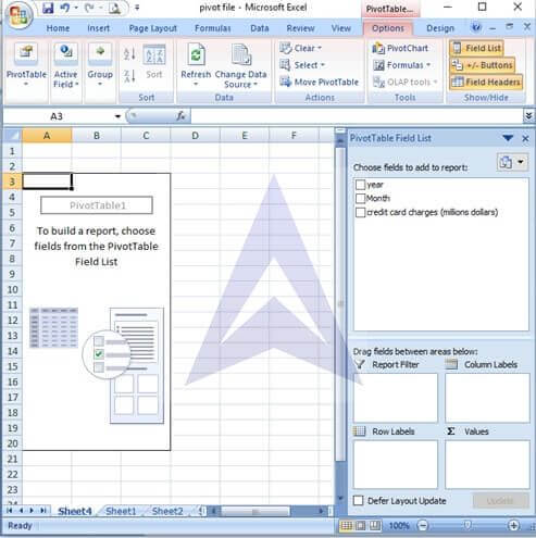
Step 4: in the right panel, drag the option Month to the section of Row Labels. Similarly drag the option of Year. Drag the option Credit Card Charges to section Values. This creates the pivot table as shown below:
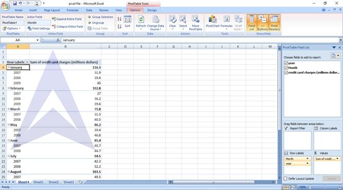
Step 5: In the Pivot table tools, go to Options -> Field Settings.
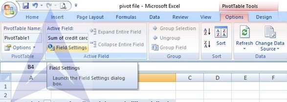
In the field settings tool box, under Summarize by, select the option ‘Average’ and under show values as, select the option of ‘% of total’. The following pivot table appears.
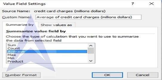
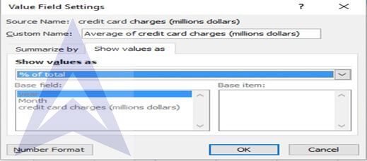
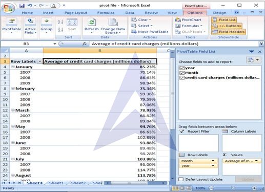
Step 6: For the purpose of pasting the monthly average seasonal index, unselect the option of years from the right panel. Copy the resultant pivot table to Sheet 1.
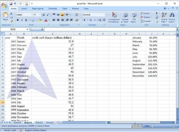
Step 7: Paste the seasonal index against the corresponding month.
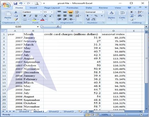
Step 8: De-seasonalize the data by dividing the credit card charges with the corresponding seasonal index.
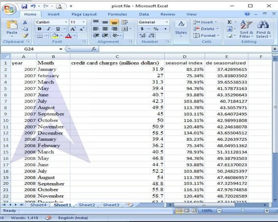
Step 9: insert a column to the left of credit card charge. In this column, number the observations.
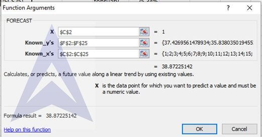
Step 10: Use the function FORECAST
{`
  Go to Formula -> More Functions -> Statistical -> FORECAST.
  In the FORECAST dialog box, enter the following:
  X: C2
  Known y’s: F2 to F25
  Known x’s : C2 to C25
  `}
The following is the final output:
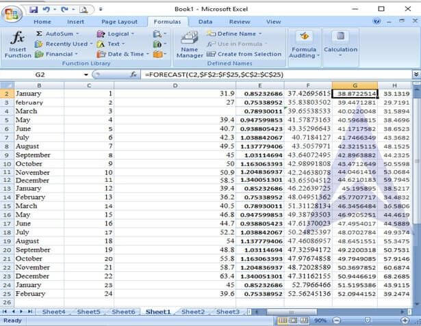
On the basis of the forecast, the value of credit card charge for February 2009 is 39.24. The actual value is 39.6. Therefore, it can be concluded that even though the charge was very high in December 2008, but, the charge in February is expected to be low because of the presence of seasonality.
E. Develop an exponential trend forecasting equation with monthly components.
Step 1: Copy and paste data on excel and take log (base 10) of credit charge.
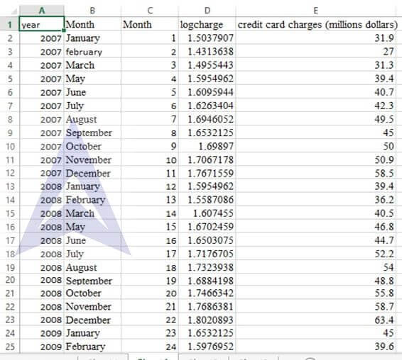
Step 2: Click on data and then click data analysis tool pack and select regression. For x values select cells C1 to C25 and for x values select cells D1 to D25. Regression summary is obtained.
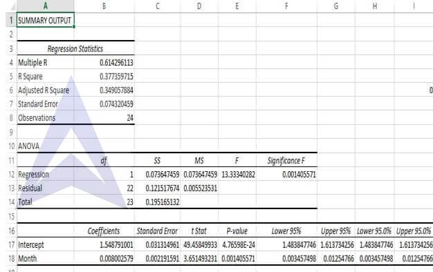
Forecast equation:
The following values can be obtained by converting the intercept value as 10^intercept and taking the Month coefficient from regression summary Y=35.38270251* 10^ (0.0080*t)
F. Interpret the monthly compound growth rate.
The monthly compound growth rate is 0.065524102 or 6.55%. This means that on an average every month the charges grow by 6.55%
G. Interpret the January multiplier
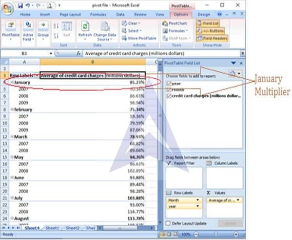
The January multiplier is 0.8523 or 85.23% every January (see Pivot table output). It mean that in the month of January, the charges are only 85.23% of the total annual average credit card charges.
H. What is the predicted value for March 2009?
{`
  Taking t= 25
  Y=35.38270251* 10^ (0.0080*t)
  =35.38270251* 10^ (0.0080*25)
  =56.07
  `}
I. What is the predicted value for April 2009?
{`
  Taking t= 26
  Y=35.38270251* 10^ (0.0080*t)
  =35.38270251* 10^ (0.0080*26)
  =57.11
  `}
J. How can this type of time-series forecasting benefit the bank?
Time-series financial forecasting can help banks in analyzing potential portfolio decisions over a time horizon. Banks can conduct prediction of the future external economic environment as well as their own internal financial variables. Bank’s current financial position depends heavily on the previous decisions of deposits and funding as well as acquiring funds out of several investment opportunities of varying returns and time horizons. These decisions will also be affected by overall external economic environment as well as future expectations of financial and economic variables as well as expected targets for meeting management objectives. All these financial planning decisions can be optimized based on time-series forecasting of relevant economic and financial variables.
Excel Econometrics Tutorials
Multiple Regression Analysis
- Estimation and Inference
- Estimation, Inference & Prediction
- Model Formation: Checking Significance of Independent Variables
Time Series Analysis
- Exponential Smoothing Forecasting
- Plotting Linear Trend and Forecasting
- Monthly Data De-Trending, Seasonal Index & Forecasting
- Linear, Exponential and Quadratic Trend
- Excel Tutorial for Normal Distributions
Data Analysis


