Correlation and Regression Assignment Help
Bivariate Distribution:
In a bivariate distribution we may be interested to find out if there is any correlation or covariation between the two variables under study. If the changes in one variable affects a change in the other variable, the variables are said to be correlated. If the two variables deviate in the same direction, that is if the increase in one results in a corresponding increase in the other, correlation is said to be direct or positive. But if they constantly deviate in the opposite direction, that is if increase in one results in corresponding decrease in the other, correlation is said to be diverse or negative.

Scatter Diagram:
It is simplest way of the diagrammatic representation of bivariate data. Thus for the bivariate distribution (xi,yi) ; i=1,2,………n. if the values of the variables X and Y be plotted along the x-axis and y-axis respectively in the xy plan, the diagram of dots so obtained is known as scatter diagram. From the scatter diagram, we can form a fairly good, though vague, idea whether the variables are correlated or not, e.g., if the points are very dense, i.e., very close to each other we should expect a fairly good amount of correlation between the variables and if the points are widely scattered, a poor correlation is expected. This method, however, is not suitable if the number of observations is fairly large.
What is a frequency distribution?
In statistics, Frequency distribution refers to the summarization of the statistical data that shows the frequencies of the values of a variable.
Correlation and Regression Assignment Help Through Online Tutoring and Guided Sessions from AssignmentHelp.Net
In other words, it is a tabular or graphical form that displays the frequencies of various outcomes in a sample.
Bivariate (“Bi” means “Two” and “variate” means “variable”) is a commonly used term that describes a data which consists of observations showing two attributes or characteristics (two variables). In other words, bivariate distribution studies two variables.
Thus, when the data set are classified (summarized or grouped in the form of a frequency distribution) on the basis of two variables, the distribution so formed is known as a bivariate frequency distribution.
Consider the following example for the Bivariate frequency distribution of two variables involving sales revenue (in $) and Advertisement expenditure (in $) of 38 firms.
| Sales Revenue | Advertisement Expenses | total | |||
|---|---|---|---|---|---|
| 20-40 | 10-30 | 30-50 | 50-70 | 70-90 | |
| 40-60 | 4 | 2 | 6 | - | 12 |
| 60-80 | 3 | 4 | 3 | 2 | 12 |
| 80-100 | 1 | 5 | 2 | 3 | 11 |
| 100-120 | - | 2 | 1 | - | 3 |
| total | 8 | 13 | 12 | 5 | 38 |
The sales revenue has been classified in different rows and the advertisement expense is shown in different columns. Each cell shows the frequency which is the number of firms corresponding to the given range of sales revenue and advertisement expenses.
CORRELATION ANALYSIS
What is Correlation?
According to Simpson & Kafka, “Correlation analysis deals with the association between two or more variables”.
Correlation tells about the degree of relationship between the variables under consideration.
The correlation coefficient or the correlation index is called the measure of correlation. It tells the direction as well as the magnitude of the correlation between two or more variables.
Types of Correlation
1. Positive Correlation
The correlation between, say, two variables is positive when the direction of change of the variables is same i.e. if as one variable increases, then the other variable also increases or if as one variable decreases, then the other variable also decreases.
2. Negative Correlation
The correlation between, say, two variables are negative when the direction of change of the variables is opposite i.e. if as one variable increases, then the other variable decreases or if as one variable decreases, then the other variable increases.
3. Linear Correlation
The correlation is linear when the amount of change in one variable with respect to the amount of change in the other variable tends to be a constant ratio. Consider an example of linear correlation.
Let there be two variables Y and Z and following relation is observed between the two:
| Y | Z |
| 10 | 20 |
| 20 | 40 |
| 30 | 60 |
| 40 | 80 |
| 50 | 100 |
Clearly, the above table shows that the ratio of change between the two variables is the same (1/2). Plotting the two variables Y and Z on a graph would show all the points falling in a straight line.
4. Non-Linear Correlation
The correlation between two variables is non-linear or curvilinear when the amount of change in one variable with respect to the amount of change in the other variable does not exhibit a constant ratio.
5. Simple, Partial and Multiple Correlation
When the relation between two variables is being studied, then it is a simple correlation.
In multiple correlations, three or more variables are studied simultaneously.
In partial correlation, though more than two variables are involved, the correlation is studied between two variables only and all other variables are assumed to be constant.
Methods of Analyzing Correlation Between Variables
SCATTER DIAGRAM METHOD
The scatter plot (or dot chart) helps us to visually decide if the two variables are correlated or not. In this method, the given data are plotted on a graph in the form of dots (X-axis shows X values and Y-axis shows Y values).The patterns shown below describes the degree (weak, moderate or strong) and direction (positive or negative) of correlation-
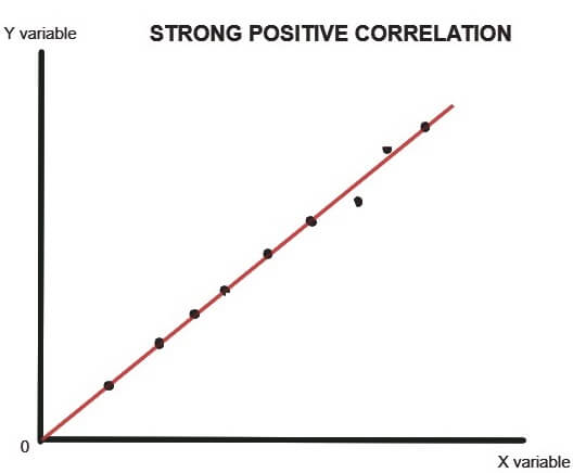
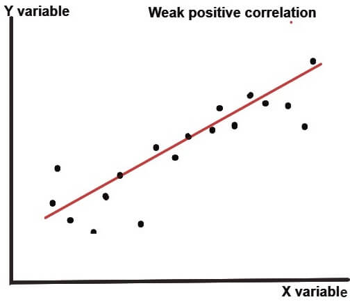
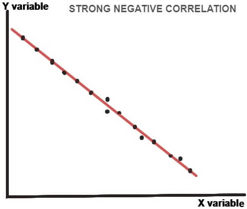
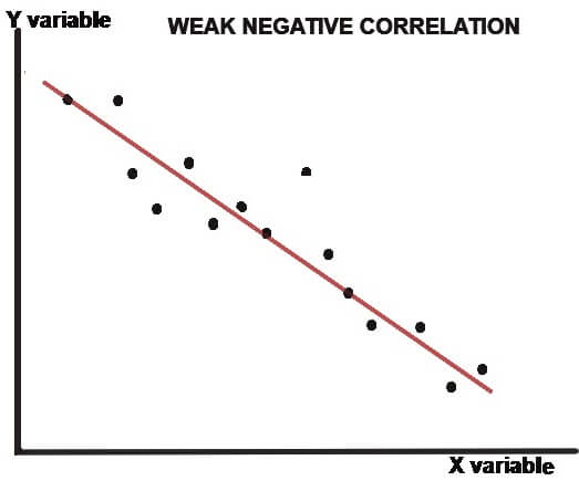
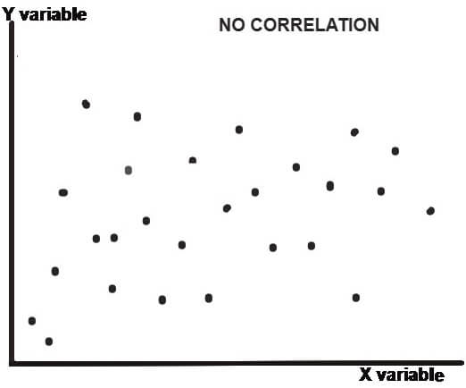
As clear from the above dot charts, the greater the scatter of the plotted points on the chart, the weaker is the relationship between two variables (X and Y). the more closely the points come to a straight line, the stronger is the degree of correlation between the variables.
When the two variables are strongly positively correlated, then the coefficient of correlation (r) is +1 i.e. r=+1 and when the correlation is strongly negative, then the coefficient of correlation is -1 i.e. r=-1.
Merits of scatter diagram method
- Simple and easy to understand. It is a non-mathematical method of studying the correlation between the variables.
- Gives a rough idea about the degree of correlation quickly.
Demerits of scatter diagram method
This method of analyzing correlation does not give the exact degree of correlation between the variables.
KARL PEARSON’S COEFFICIENT OF CORRELATION
Karl Pearson’s method of measuring correlation is most widely used in practice. It is also known as the product-moment coefficient of correlation.
The coefficient of correlation is denoted by r and denotes the degree of correlation between the two variables.
The important assumptions of the Pearsonian Coefficient of correlation are that there is a linear relationship between the variables under study and this method can be used only when the population being studied is normally distributed.
When deviations are taken from actual mean
When deviations are taken from actual mean, the formula used for computing Pearsonian coefficient of correlation (r) is-
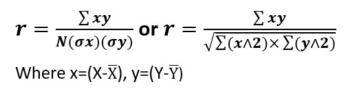
σx = Standard deviation of series X
σy = Standard deviation of series Y
N = Number of pairs of observations
r = The correlation coefficient
The coefficient of correlation not only describes the magnitude of correlation, but also the direction of the correlation.
The value of coefficient of correlation that is achieved from the above mathematical formula (only when deviations are taken from actual mean and not from assumed mean or any arbitrary number) shall lie between -1 and +1.
The coefficient of correlation denoted by r is a pure number. Changing the scale does not affect its value. This means that if a given series is divided or multiplied by some constant amount, then the r would not be affected by such a change of scale in the series.
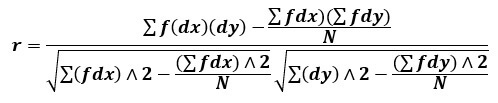
When deviations are taken from an assumed mean (arbitrary number)
When deviations are taken from assumed mean, then the following formula is used-
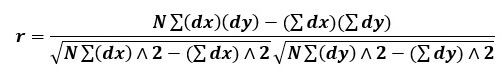
Where, dx refers to deviations of X series from an assumed mean i.e. (X-A)
dy refers to deviations of X series from an assumed mean i.e. (Y-A)
∑(dx)(dy) = Sum of the product of deviations of X and Y series from their assumed means
∑(dx)∧2 = Sum of the squares of the deviations of X series from an assumed mean
∑(dy)∧2 = Sum of the squares of the deviations of Y series from an assumed mean
∑(dx) = sum of the deviations of X series from an assumed mean.
∑(dy) = sum of the deviations of Y series from an assumed mean.
Correlation of Grouped data
When the number of observations is large, then the data is classified into different classes (continuous class intervals) or discrete items with respective frequencies. In this case, we have to create a two-way frequency distribution known as bivariate frequency table or correlation table. The formula for calculating the coefficient of correlation is-
The above formula is same as the formula for the assumed mean. The only difference is that the deviations are multiplied by frequencies (and the numerator and the denominator have been divided by N).
SPEARMAN’S RANK CORRELATION COEFFICIENT
When the correlation is calculated by ranking the observations according to size and basing the calculations on the ranks rather than upon the original observations, then we get what is called coefficient of rank correlation.
The spearman’s rank correlation coefficient is defined as-
R = 1 - 6 ∑(D ∧ 2) / (N ∧ 3)- N
Where R denotes rank coefficient of correlation and D denotes the difference of ranks between paired items in two series.
When R=+1, then there is complete agreement in the order of the ranks and the ranks are in the same direction.
When R=-1, then there is complete disagreement in the order of the ranks and the ranks are in opposite direction.
There can be three types of problems in rank correlation-
a. When ranks are given
EXAMPLE- Seven methods of imparting education were ranked by students of two university A and B.
| Method of teaching | Ranks by students of Univ. A | Ranks by students of Univ. B |
|---|---|---|
| 1 | 2 | 1 |
| 2 | 1 | 3 |
| 3 | 5 | 2 |
| 4 | 3 | 4 |
| 5 | 4 | 7 |
| 6 | 7 | 5 |
| 7 | 6 | 6 |
Calculate rank correlation coefficient.
SOLUTION- Let the ranks by students of Univ. A be denoted as RA and ranks by students of Univ. A be denoted as RB.
| Method of teaching | RA | RB | D2= (RA-RB)2 |
|---|---|---|---|
| 1 | 2 | 1 | 1 |
| 2 | 1 | 3 | 4 |
| 3 | 5 | 2 | 9 |
| 4 | 3 | 4 | 1 |
| 5 | 4 | 7 | 9 |
| 6 | 7 | 5 | 4 |
| 7 | 6 | 6 | 0 |
R = 1 - 6∑(D∧2) / (N∧3)-N
R = 1 - 6×28 / (7×7×7)-7
R=1-0.5
R=+0.5
b. When ranks are not given
When the actual data are not given, then the ranks have to be assigned. Ranks can be assigned by taking 1 as the highest or the lowest.
EXAMPLE- Consider the following data
| Y | Z |
|---|---|
| 53 | 47 |
| 98 | 25 |
| 95 | 32 |
| 81 | 37 |
| 75 | 30 |
| 61 | 40 |
| 59 | 39 |
| 55 | 45 |
Calculate spearman’s rank correlation coefficient.
SOLUTION- first we will have to assign the ranks. This is shown below-
| Y | R1 | Z | R2 | (R1-R2)2 = D2 |
|---|---|---|---|---|
| 53 | 1 | 47 | 8 | 49 |
| 98 | 8 | 25 | 1 | 49 |
| 95 | 7 | 32 | 3 | 16 |
| 81 | 6 | 37 | 4 | 4 |
| 75 | 5 | 30 | 2 | 9 |
| 61 | 4 | 40 | 6 | 4 |
| 59 | 3 | 39 | 5 | 4 |
| 55 | 2 | 45 | 7 | 25 |
| ∑(D∧2) = 160 |
R = 1 - 6∑(D∧2)) / (N∧3)-N
R = 1 - 6×160 / (8×8×8)-8
R=1-1.905
R=0.905
c. When ranks are equal
There may be cases when two or more observations have to be assigned equal ranks. When equal ranks are assigned to some observations, then following adjustments must be made in the above-stated formula-
Where m stands for the number of items with common rank. This value is added as many times as the number of such groups.
EXAMPLE- Consider the following data
| Y | Z |
|---|---|
| 15 | 40 |
| 20 | 30 |
| 28 | 50 |
| 12 | 30 |
| 40 | 20 |
| 60 | 10 |
| 20 | 30 |
| 80 | 60 |
Calculate Spearman’s rank correlation coefficient.
SOLUTION-
| Y | R1 | Z | R2 | (R1-R2)2 = D2 |
|---|---|---|---|---|
| 15 | 2 | 40 | 6 | 16 |
| 20 | 3.5 | 30 | 4 | 0.25 |
| 28 | 5 | 50 | 7 | 4 |
| 12 | 1 | 30 | 4 | 9 |
| 40 | 6 | 20 | 2 | 16 |
| 60 | 7 | 10 | 1 | 36 |
| 20 | 3.5 | 30 | 4 | 0.25 |
| 80 | 8 | 60 | 8 | 0 |
| ∑(D∧2) = 81.5 |
- 20 has been ranked 3.5 ((3+4)/2) and 30 has been ranked as 4 ((3+4+5)/3)
- Item 20 has repeated 2 times in the Y series. Item 30 in Z series has occurred 3 times. So, we take m value to be 2 and 3.
Merits of Rank Correlation Method
- This method is simple to understand as well as easy to apply than Karl Pearson’s rank correlation method.
- This method is useful when the data is of qualitative nature. Karl Pearson’s method can be used only for the data of quantitative nature.
Demerits of Rank Correlation Method
- This method cannot be used for finding correlation when we have a grouped frequency distribution.
- When the no. of observations in a data set are very large (usually greater than 30), then the calculation becomes tedious and time-consuming.
REGRESSION ANALYSIS
According to Morris Hamburg “The term ‘regression analysis’ refers to the method by which estimates are made of the values of a variable from the knowledge of the values of one or more other variables and to the measurement of the errors involved in this estimation process.”
In other words, Regression analysis is a statistical device with the help of which we can estimate the unknown values of one variable from known values of another variable.
The variable which is predicted is known as dependent variable while the variable which is used to predict the dependent variable is known as an independent variable.
The regression analysis carried here is called simple linear regression analysis. In this type of regression, there is only one independent variable and there is a linear relationship between the dependent variable and independent variable.
Regression line in case of the simple linear regression model is a straight line that describes how the dependent variable Y (or response variable) changes as the explanatory variable X (or predictor variable) changes.
While the correlation between X and Y tells about the degree of relationship between the two variables, the regression analysis helps in understanding the nature of relationship so that the values of the dependent variable (Y) can be predicted on the basis of the fixed values of the independent variable (X).
Regression Equations
Regression equations are the algebraic expressions of regression lines.
There are two types of regression equations:
a. Regression equation of Y on X
Here, X is an explanatory variable and Y is a dependent variable. This type of regression equation describes the variations in Y values for given changes in X. the equation is expressed as follows:
Ŷ = a + bX
- Ŷ is the computed (estimated) value of dependent variable. (It is different from the actual value of Y by the amount of error in prediction).
- a is the intercept which tells the value of Y (dependent variable) when X (explanatory variable) is Zero. The interpretation of intercept may not always make scientific sense.
- b determines the slope of the regression line representing the above equation. It tells the change in Y due to a given small change in X.
b. Regression Equation of X on Y
Here, Y is an explanatory variable and X is a dependent variable. This type of regression equation describes the variations in X values for given changes in Y. The equation is expressed as follows:
X̂ = a + bY
- X̂ is the computed value of dependent variable. (It is different from the actual value of X by the amount of error in prediction).
- a is the intercept which tells the value of X (dependent variable) when Y (explanatory variable) is Zero. The interpretation of intercept may not always make scientific sense.
- b determines the slope of the regression line representing the above equation. It tells the change in X due to a given small change in Y.
The simple regression analysis calculates the parameters a and b using the approach of ordinary least squares (OLS). According to this approach, the regression line should be drawn in such a way that the sum of squares of the deviations of the actual Y values from the computed Y values is the least i.e. ∑(Y-Ŷ)2 must be minimum.
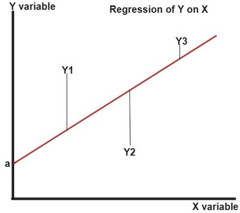
The above figure shows the sample regression line (Y on X) of best fit (shown by red line) which plots the computed values of Y (Y ̂)for given values of X values. Y1, Y2 and Y3 are the actual values of the variable Y. The vertical distances between the actual value of variable Y (Y1, Y2 and Y3) and computed value of Y gives the residuals (error term). The approach of ordinary least square states that these errors (or residuals) must be minimum. The least square line (in the figure above) is the best estimate of the population regression line.
FINDING REGRESSION EQUATION
One way of finding regression equation is using Normal equations.
As we know that the regression equations of Y on X are given by: Ŷ = a + bX
In order to find the values of a and b in case of regression of Y on X, we use following two normal equations:
∑Y = Na + b∑X
∑XY = a∑X + b∑X2
The values of a and b can be found out by solving the two above normal equations simultaneously.
As we know that the regression equations of X on Y are given by: X̂ = a + bY
In the case of regression of X on Y, we use following two normal equations to calculate a and b:
∑X = Na + b∑Y
∑XY = a∑Y + b∑Y2
When deviations are taken from Arithmetic means of X and Y
The above method of finding out the regression equation is cumbersome. Instead, we can use the deviations of X and Y observations from their respective averages.
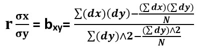
1. Regression equation of X on Y
The regression equation of Y on X can also be expressed in the following form-
X - X̅ = r σx/σy (Y-Y̅)
Here, X̅ is the average of X observations and Y̅ is the average of Y observations.
r σx/σy is the regression coefficient of X on Y and is denoted by bxy. bxy measures the amount of change in X corresponding to a unit change in Y.
r σx/σy = bxy = ∑xy/∑y∧2
Where x=(X-X̅) and y=(Y-Y̅)
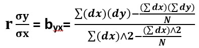
2. Regression equation of Y on X
The regression equation of Y on X can also be expressed in the following form-
Y - Y̅ = r σy/σx(X - X̅)
r σy/σx is the regression coefficient of Y on X and is denoted by byx. byx measures the amount of change in Y corresponding to a unit change in X.
r σy/σx = byx = (∑xy)/∑x∧2
We can calculate the coefficient of correlation which is the geometric mean of the two regression coefficients (bxy & byx) i.e.
r = √(bxy)×(byx)
Some of the important properties of the regression coefficients are as follows-
- Regression coefficients are independent of the change of origin but are not independent of the change of scale.
- Both the regression coefficients (bxy & byx) have the same sign i.e. if bxy is positive then byx will also be positive and vice versa.
- The correlation coefficient is the geometric mean of the two-regression coefficient (as shown above).
- As the value of the correlation coefficient cannot exceed unity, one of the regression coefficients has to be less than one if the other coefficient is greater than 1.
- The coefficient of correlation will always have the same sign as that of regression coefficients.
When deviations are Taken from Assumed Mean
When instead of using actual means of X and Y observations, we use any arbitrary item (in the observation) as the mean.
We consider taking deviations of X and Y values from their respective assumed means.
The formula for calculating regression coefficient when regression is Y on X is as follows:
Where dx = (X-Ax) {Ax = assumed mean of X observations} and dy = (Y-Ay) {Ay = assumed mean of Y observations}
The formula for calculating regression coefficient when regression is X on Y is as follows:
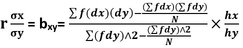
In the case of Grouped frequency distribution, the regression coefficients are calculated from the bivariate frequency table (or correlation table).
The formula for calculating regression coefficient (in case of grouped frequency distribution) when regression is of Y on X is as follows-
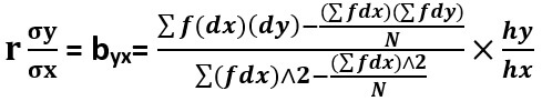
Where hx = class interval of X variable And hy = class interval of Y variable
The formula for calculating regression coefficient (in case of grouped frequency distribution) when regression is of X on Y is as follows-
STANDARD ERROR OF ESTIMATE
The standard error of estimate is a measure of the accuracy of a prediction made using regression line.
It is not possible to exactly estimate (or predict) the values of the dependent variable. For example The estimate about the amount of agricultural produce (Y) depending upon the amount of rainfall (X) that the country receives in a year can be approximately close to the actual figures, but the prediction cannot be exact (rare cases being exceptions).
The standard error of estimate helps in measuring the dispersion (or variation) about the estimated regression line. If standard error is zero, then there is no variation about the regression line and the correlation will be perfect.
We can calculate the standard error of regression of values from Ŷ through the following formula-
Syx = √∑(Y-Ŷ) / N (Regression of Y on X)
Or, Syx = σy√1-r2
∑(Y-Ŷ) = Unexplained variation i.e. the variation in the Y values that cannot be explained by the regression model.
We can calculate the standard error of regression of values from X̂ through the following formula-
Sxy = √∑(X-X̂) / N (Regression of X on Y)
Or, Sxy = σx√1-r2
∑(X-X̂) = Unexplained variation i.e. the variation in the X values that cannot be explained by the regression model.
LIMITATIONS OF REGRESSION ANALYSIS
While estimating a variable from the regression equation, it is assumed that the cause and effect relationship between the two variables remain unchanged. This assumption may not be always satisfied and hence estimation may be misleading.
Also, the regression analysis discussed above cannot be used in case of qualitative variables like honesty, crime etc.
Email Based Homework Help in Correlation and Regression
To submit Correlation and Regression assignment click here.
Following are some of the topics in Correlation and Regression in which we provide help:
- Bivariate Normal Distribution
- Multiple And Partial Correlation
- Plane Of Regression
- Properties If Residuals
- Coefficient Of Multiple Correlation
- Properties Of Multiple Correlation Coefficient
- Coefficient Of Partial Correlation
- Multiple Correlation In Terms Of Total And Partial Correlation
- Coefficient In Terms Of Regression
- Expression For Partial Correlation