How to do an OLS multiple linear regression in STATA
Using OLS, let us estimate the parameters in a simple model where LNWAGE is regressed on a constant, years of schooling (EDU), and experience (EX) and report these along their estimated standard errors. What do the slope coefficients on EDU and EX measure? Intuitively, age may affect as well. What would be the problem of including AGE as an additional regressor?
MULTIPLE LINEAR REGRESSION IN STATA (Only Quantitative Independent Variables)
Using STATA, we estimate the following equation: LNWAGE = C + β1EDU + β2EX
The natural logarithm of average hourly wage earning in dollar (LNWAGE) is the regressand,
C refers to a constant term in the regression equation,
Years of education (EDU) and potential years of experience (EX) are the regressors.
Using ordinary least square method (OLS) of estimation, we regress LNWAGE on a constant, years of schooling and experience. The command for STATA for conducting multiple linear regression in STATA is:
{`
  Regress Independent Variable Dependent variable1 Dependent variable2 Dependent Variable3…….
  `}
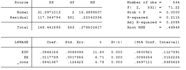
The STATA command for this problem is given below and the regression output obtained is as follows:
{`Regress LNWAGE EDU EX`}

Interpretation of Multiple Linear Regression Output from STATA
The slope coefficient corresponding to years of education (EDU) implies that one unit change in years of education leads to 9.64% change in average hourly earnings in same direction (indicated by a positive sign with the coefficient), given all other variables are kept unchanged.
Similarly, the slope coefficient corresponding to potential years of experience (EX) implies that one unit change in potential years of experience leads to 1.17% change in average hourly earnings in the same direction ( indicated by a positive sign with the coefficient), given all other variables are kept unchanged.
The estimated value of constant term can be interpreted as the minimum hourly wage earnings in dollar obtained by an individual with no education and experience. Thus, individual with absolutely no education and experience derives an hourly wage equals to antilog (0.5941).
The standard errors in output table indicate dispersion in estimated values around the average, in the distribution of the variable being considered. The standard error value of 0.0083 corresponding to variable EDU indicates that when repeated samples are drawn, 95% of times the estimated years of education will lie within 0.0166 (2 times standard error, which is 0.0083) of true years of education. Lower standard errors corresponding to all the coefficients indicate that the estimated values are close to the actual values.
The value of z- statistic corresponding to all coefficients is greater than 2 in absolute value, thus we reject the null hypothesis that the corresponding beta coefficient is 0. It means, we do not reject the alternative hypothesis that the corresponding beta coefficient is unequal to 0. Thus, the beta coefficients are all statistically significant at 5% level of significance. Also, the p-value corresponding to all the beta coefficients is less than 0.05, which indicates the statistical significance of all beta coefficients.
Intuitively, age may affect the hourly wage earnings in dollar as well. There will be a problem of auto correlation if age is added as another regressor in regression equation. This is because the variable EX measuring potential years of experience is already obtained using age as one of its component. Adding age as a separate variable will result in auto-correlation as regressors EX and Age will be correlated and as a result Gauss Markov Assumption of no autocorrelation will be violated and the model will not be correctly specified.
QUADRATIC REGRESSION MODEL IN STATA
Because human capital depreciates with age (and hence with the measure of experience we are using), we expect decreasing returns to experience. To see whether this assumption is correct, estimate a linear model with the additional quadratic in experience variable: LNWAGE = β0 + β1EDU + β2EX + β3EXSQ + ε
Is the sign of β3 consistent with what you expect? Is β3 statistically significant? At what level of experience is LNWAGE maximized? What happens to the estimated coefficients of EDU and EX and their standard errors?
Assumption: Diminishing returns to experience as human capital depreciates with age (and hence with the measure of experience we are using) To test this assumption, we estimate the following linear model with additional quadratic in experience variable; LNWAGE = β0 + β1EDU + β2EX + β3EXSQ + ε
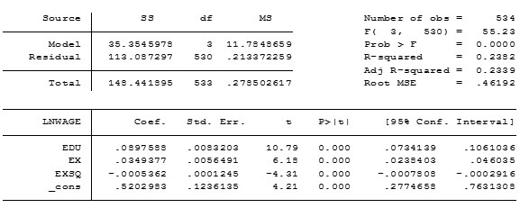
In STATA, the regression output along with commands in bold is given as:
{`Regress LNWAGE EDU EX EXSQ`}

We expect diminishing returns to experience. Thus with every unit increase in potential experience, the LNWAGE should increase at a diminishing rate. The negative sign of β3 indicates that relationship between experience and LNWAGE is concave to the origin, which in turn implies that for every unit increase in experience, the LNWAGE also rises but at a diminishing rate due to concavity. Therefore the sign of β3 is in agreement with our expectation.
Since z-value corresponding to β3 is greater than 2 in absolute value, we reject the null hypothesis that β3=0 and does not reject the alternative hypothesis that β3 not equals 0 at 5% level of significance. Therefore, the quadratic variable of experience is statistically significant at 5% level of significance. Also, p-value corresponding to quadratic variable of experience (EXPSQ) is less than 0.05, it indicates the statistical significance of EXPSQ in the regression equation at 5% level of significance.
To estimate the level of experience (EX) which maximizes LNWAGE, we differentiate the model with respect to experience and first order condition obtained is set equal to zero.
The first order condition obtained is: f ‘ = Β2 +2*β3EX = 0
Solving this equation gives;
EX = -β2/2* β3 , then plug the value of beta coefficients and we obtain EX = 32.5789 years. To ensure that this value of EX maximizes LNWAGE, we differentiate the first order condition and second order differential equation is obtained as under: f ”= 2*β3, since sign of β3 is negative the sign of second order differential is also negative and this ensure maximization of LNWAGE at this level of EX.
With the inclusion of quadratic of EX in the regression model, the coefficient of EX has increased from 0.0112 to 0.0349 and that of EDU has fallen from 0.09641 to 0.08975.
The standard error corresponding to EDU has remained almost unchanged with slight movement from value of 0.008309 to 0.008320.
The standard error corresponding to EX has increased from 0.00175 to 0.00564.
Lastly, the constant term in the model has decreased from 0.59413 to 0.52029 and standard error has fallen slightly from 0.12444 to 0.12361.


