STAT20029 Module 4: Probability
Introduction
This week we explore the topic of probability. This material is a foundation for much of the remainder of the Assignment and so it is important that it is learned well. Probability is a topic that is used often in everyday life, having applications everywhere from the court room to medical drug trials, from weather forecasting to the stock exchange. Because of the widespread use (and misuse) of probability, it is important for us to consider how to ethically and professionally employ these techniques in the workplace. Probability is a branch of statistics which can be considered as the toolkit of statistics.
Objectives
On completion of this module you should be able to:
- demonstrate understanding of basic probability concepts including sample spaces, events, contingency tables, marginal and joint probability
- use and compute conditional probabilities
- use the addition and multiplication rules
- explain and demonstrate statistical independence and
- apply Bayes’ theorem and counting rules.
Basic Probability
What is probability?
Probability is the likelihood or chance that a particular event will occur. An event that is certain has a probability of 1. An impossible event has a probability of 0. All probabilities are values from 0 to 1 (inclusive). A probability value under no circumstances whatsoever can be greater than one or be a negative number.
The event we are interested in is described by a capital letter, such as E (for event), or sometimes some more meaningful letter. For example, if we are interested in whether it rains today, we might define R = the event that it rains today. The probability of an event is denoted by [or for the rain example]. If X is a variable with several possible outcomes and we seek the outcome E, then the probability is written as P(X=E).
Three approaches to probability
Classical probability—the probability of success is based on prior knowledge or intuition of the process involved. This kind of approach to probability is sometimes referred to as the relative frequency of occurrence. The probability of occurrence of an event, E, is found via:
Example
A six-sided die has six possible outcomes. Therefore, the probability of rolling a five is 1/6.
If two dice are rolled, there are 6 × 6 = 36 possible outcomes. The probability of rolling a total of six (adding the two values together) is 5/36 since you could roll 1 & 5, 2 & 4, 3 & 3, 4 & 2 or 5 & 1.
The die for this experiment is considered to be fair – it has uniform density, the edges are of equal length, and each surface is smooth and flat.
Empirical probability—probabilities are based on observed data, not on intuitive knowledge of the process. This method may involve an experiment to produce outcomes. The probability of occurrence of an event, E, is found via:
P(E)=Number of outcomes in which event occurs /Total number of outcomes
Example
If we observed that one out of five cars in a car park is white, we could say that the probability that the next car that enters the car park is white is 1/5.
Subjective probability—the chance of an event is assigned by a particular individual or group. This means that different people may assign different probabilities. Probabilities are based on the feelings or insights of the person determining the probability. It ranges from a guess as a worst case to accurate probabilities (particularly where the person has knowledge, understanding and experience of the event). Subjective probability is useful when probabilities of events can’t be determined empirically. An example might be that a doctor could assign a fairly accurate probability on the life expectancy of a cancer patient. Another example could be that a punter, who has carefully observed all the horses, places a wining bet on a horse he thinks has the highest probability of winning. Subjective probability is a method of capturing the knowledge of a talented experienced person.
Some definitions
An event—a possible type of occurrence or the outcome of an experiment. For example, rolling a six on a single die or there is rain on Tuesday.
A simple event—can be described by a single characteristic. It is different from elementary event where the event cannot be decomposed into smaller events.
Sample space—the collection or list of all possible events.
Complement—the complement of an event A, written A', is all the events which are not part of the event A. Since the event must either occur or not occur, we can say that (A)+P(A' )=1..
Joint event—an event that has two or more characteristics.
Contingency table—a table of cross-classifications.
Simple (marginal) probability—the probability of occurrence of a simple event.
Joint probability—a probability referring to two or more events.
Important note: to be statistically correct, and because probability is always a number between 0 and 1 (inclusive), answers to probability questions should also be expressed as values between 0 and 1, and if desired, it can be expressed as percentages between 0% and 100%.
Addition rules
If two events A and B are being considered, the probability of either of the events occurring is given using the following general addition rule:
P(A or B)=P(A)+P(B)-P(A and B)
Mutually exclusive events are events where the occurrence of one means that the other(s) cannot occur. For example, the variable of gender results in mutually exclusive outcomes. A person is either male or female, not both. In manufacturing, whether a product is good or defective are mutually exclusive outcomes.
If two events, A and B, are mutually exclusive, then the probability of either of the events occurring is found using the following addition rule for mutually exclusive events:
P(A or B)=P(A)+P(B), since.
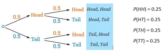
Probability tree diagram
A tree diagram is another method of delineating the sample space. It also describes pathways in which an event can occur. Each branch of the tree gives the probability of moving from the left node to the right node of that branch. The probability of an event occurring at a node is equal to the value obtained by multiplying all the probability values of previous branches leading to that node. The probability tree diagram of a coin being tossed twice is given in the figure below:
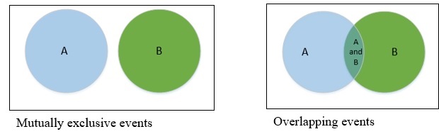
Venn diagram
A Venn diagram is a pictorial way of depicting relationships between events and sample space. Usually the sample space is represented by a rectangle and events by circles. The common elements are represented by overlapping areas of circles.
|
Example 4–1 A store manager is interested in whether repeat customers spend more money in his store than first-time customers do. He takes a random sample of 200 customers over a one-month period with the following results:
(a) Give an example of a simple event. (b) Give an example of a joint event. (c) What is the complement of ‘new customer’? (d) Why is ‘new customer who spent over $200’ a joint event? If a customer is selected at random, what is the probability that he or she (e) is a new customer? (f) spent $200 or less? (g) is not a new customer and spent over $200? (h) is not a new customer or spent over $200? (i) Explain the difference between your answers to (g) and (h). |
Conditional probability
Conditional probability
Conditional probability is the probability that an event will occur, given that another event has already happened. It is expressed as P(A|B) which is read as ‘the probability of A given B’. This probability is found via:
P(A|B)=P(A and B)/P(B)
Note this rule applies only if P(B)≠0. If you draw the Venn diagram, you will find that the conditional probability is tantamount to reducing the sample space to event B only.
Statistical independence
Independent events are events when the occurrence of one event has no effect on the probability that another will occur. Dependent events means that when one event occurs, this changes the probability that another will occur. In order to demonstrate statistically that two events are independent, we use the following rule.
Two events are statistically independent if and only if P(A|B)=P(A). The vertical line indicates “given that”, the whole expression to the left means probability of A given that B has already occurred. It is intuitive to think of independent events in terms of a sequence of experiments, where the outcome of an experiment does not affect the possible outcome of the next experiment.
Multiplication rules
When events A and B are independent, the probability P(A and B) can be found via:
P(A and B)=P(A)P(B).
When events A and B are not independent, the probability can be found via:
P(A and B)=P(A|B)P(B).
Events cannot be both independent and mutually exclusive because when mutually exclusive, P (A and B) = 0.
Thus, P(A│B)=(P(A and B))/(P(B))=0/(P(B))=0, which is not equal to P(A) as required to be independent.
Example 4–2
Using the table in Example 4–1 above, answer the following questions:
(a) Given that a customer spent over $200, what is the probability that he or she is a new customer?
(b) Given that a customer is new, what is the probability that he or she spent over $200?
(c) Explain the difference in your answers for (a) and (b).
(d) Are the two events, new customer and customer spent over $200 statistically independent?
Example 4–3
Chief Executive Officers (CEOs) of companies are demonstrating increasing mobility between companies. A concerned employer at a particular company worries that constantly changing the CEO in his company has left an unstable work environment for staff, and customers confused by ever changing products. He conducts a survey of 150 large companies, looking at whether the companies’ profit levels have increased or decreased and whether the company has had a new CEO within the last five years. Based on his survey he discovers that of the 150 companies, 67 have reported decreased profits. A total of 31 of the companies have not replaced their CEO within the last five years and of these, 29 have increased their profits.
Produce a contingency table summarising this information and use it to find the probability that a company has increased its profit given that it has replaced its CEO in the last five years.
Bayes’ theorem
Bayes’ theorem was developed by Thomas Bayes in the 1700s. It allows information about a second event to be used to revise the probability that a first event has occurred. It extends the conditional probability ideas that we have explored so far. In simple words, if we know P(A|B), Bayes’ theorem provides a way to calculate P(B|A).
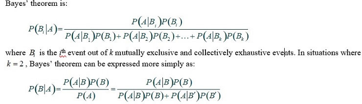
Bayes’ theorem is:
In this Assignment, we are mostly interested in using Bayes’ theorem for two events (i.e., for ).
You may have noticed that it is a universally accepted convention to write mathematical symbols in italics. Thus, “a” is a word, but “a” is a symbol.
Example 4–4
Two large supermarket chains, ‘Value Mart’ and ‘Goldies’, have been fiercely competitive with their range of products. Data are collected by an external watchdog which indicates that when a new product is introduced to the market, Goldies will begin to retail that product 90% of the time. If Goldies has already begun to market a product, Value Mart will take up the product 85% of the time. When Goldies does not begin to retail a product, Value Mart begins to retail it 25% of the time.
(a) Determine the probability that Goldies will market a product given that Value Mart is already retailing it.
(b) Find the probability that Value Mart retails a given product, .
(c) Why might this information be useful?
Counting rules
Counting rule 1
For k events (mutually exclusive and collectively exhaustive) which can occur in each of n trials, the number of possible outcomes is kn.
Example
A standard dice has six possible outcomes (k = 6). These are
mutually exclusive—there is no overlap between outcomes (for example, you cannot roll both a 1 and a 2 on the same dice at the same time!)
collectively exhaustive—there are no other possible outcomes (the only possible outcomes are 1 to 6)
If a dice is rolled once, there are six possible outcomes {1, 2, 3, 4, 5, 6 }; if the dice is rolled twice, there are 62 = 36 possible outcomes {(1, 1), (1, 2), (1, 3), (1, 4), (1, 5), (1, 6), (2, 1) ... (6, 6) } ; if the dice is rolled three times, then n = 3 there are 63 = 216 possible outcomes.
Counting rule 2
For k1 events on the first trial, k2 on the second trial, … and kn on the nth trial, then the number of possible outcomes is
k1´ k2 ´…´ kn.
Example
A courier must travel between three drop-offs in the following order: A, B and C. From A, there are two ways to reach B (). From B, there are four ways to C ().
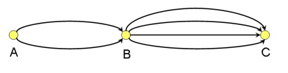
There are k1×k2=2×4=8 ways of travelling from A to C.
Counting rule 3
The number of ways that n objects can be arranged in order is n!=n×(n-1)×(n-2)×…×2×1
n! is read ‘n factorial’. We define 0! = 1 and 1! = 1.
Example
The number of ways you can arrange five cars in five parking spaces is 5!=5×4×3×2×1=120.
This means there are five ways you can allocated a car to the first parking space, and then four are left to be allocated to the second space, three for the third, two for the fourth and finally only one is left to be allocated to the fifth parking space.
Counting rule 4
Permutations—the number of ways of arranging X objects selected from n objects in order is 〖(n)P〗X=n!/(n-X)!
Example
The number of ways you can seat six people in three chairs is:
〖(6)P〗3=6!/(6-3)!=(6×5×4×3×2×1)/(3×2×1)=720/6=120 ways.
You can fill the first chair with anyone of the 6 persons. Once the first chair is occupied, you can fill the second chair with anyone of the remaining 5 persons, and so on. To explain it in further detail, consider 3 persons to sit in three chairs. The persons are named A, B, and C. You can fill the first chair with A or B or C, next you can fill the second chair with 2 remaining persons, and the last chair with the last person. The total number of possibilities is 3! = 3(2)1 = 6. The six permutations are {ABC, ACB, BAC, BCA, CAB, CBA }. There are no other possibilities.
Counting rule 5
Combinations—the number of ways of arranging X objects selected from n objects irrespective of order is ((n@X))=〖(n)C〗X=n!/X!(n-X)!
Example
The number of ways you can choose three people from a group of six to be members on a committee irrespective of order is (■(6@3))=〖(_^6)C〗_3=6!/3!(6-3)!=720/(6×6)=20 ways.
Note the difference between permutations and combinations. In combinations, order does not matter. Since you can arrange 3 people in 3! different ways, this term has to be taken out from the permutation expression.