SAP HANA Data Modeling Case Study

Step 1: Create the database tables

1. Logon to the SAP HANA Studio

Start → All Programs → SAP HANA → SAP HANA Studio

2. Create a database table for the customer master data

Navigator View → Catalog → GBI_XXX → Tables → Right click → New Table

Enter Table Name, Field Name, SQL Data Type and Dim (Field Length) as shown in the screenshot:

3. Create a database table for the product master data

Navigator View → Catalog → GBI_XXX → Tables → Right click → New Table

Enter Table Name, Field Name, SQL Data Type and Dim (Field Length) as shown in the screenshot:

4. Create a database table for the sales transaction data

Navigator View → Catalog → GBI_XXX → Tables → Right click → New Table

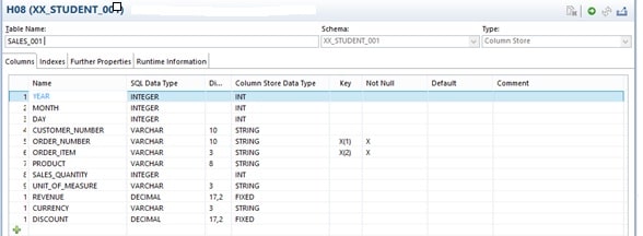
Enter Table Name, Field Name, SQL Data Type and Dim (Field Length) as shown in the screenshot:

Step 2: Data Provisioning

1. Open the modeler perspective in the SAP HANA Studio

Window → Open Perspective → SAP HANA Modeler

2. Add a new Remote Source to the SAP HANA System

Navigator View → Provisioning → Remote Sources

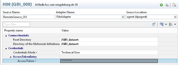
Right-click on Remote Sources, select “New Remote Source” and enter the data as shown in the screenshot. Please type in gbi as AccessToken.

3. Add virtual Data Tables to the SAP HANA System

Navigator View → Provisioning → Remote Sources → <Source Name>

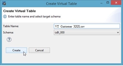
Right-click on the Customer.csv table and select “Add as virtual table”. Add “VT_” as prefix of the table name, select your Database Schema and click on create:

Repeat this step for the Product.csv and Salesdata.csv file:

4. Create a new Repository Workspace for the SAP HANA System

First, switch to the SAP HANA Development Perspective:

Window → Open Perspective → SAP HANA Development

Afterwards, right-click within the Project Explorer and navigate to the following path:

New → Other → SAP HANA → Repository Workspace

There, select your system and determine a Workspace Name and Root:

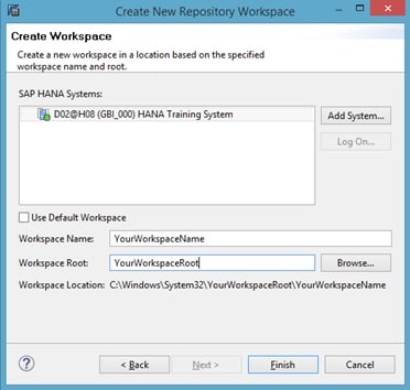
5. Create a new Repository Package within your Repository Workspace

Within the Repository View, right click on your Repository Workspace and navigate to

New → Repository Package

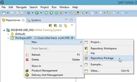
There, specify a Repository Package Name and click on Finish:

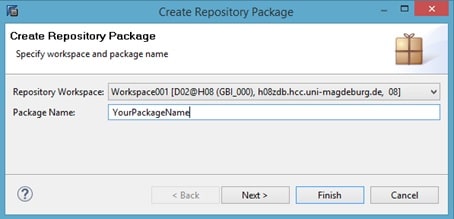
6. Within your Repository Package, create a new Flowgraph Model

Right-click on your newly created Repository Package and select

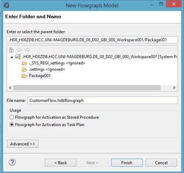
New → Other → SAP HANA → Database Development → Flowgraph Model

There, enter a name, select “Flowgraph for Activation as Task Plan” and click on Finish:

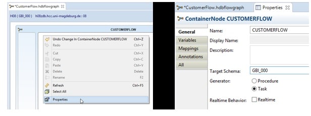
After the Loading process finished, right-click on the initially empty flow graph, select “Properties” and there, change the Target Schema to your Schema:

7. Within the Flowgraph Model, establish a data connection between the Virtual Table and the Data Table

Insert the Virtual Table “VT_Customer.csv” and the Table CUSTOMER_ATTR_XXX into the Model via Drag-and-Drop from the Table Catalog.

Determine the “VT_Customer.csv”-table as Data Source and the CUSTOMER_ATTR_XXX-Table as Data Sink.

Furthermore, create a connection between the two tables, by linking Data Source and Data Sink.

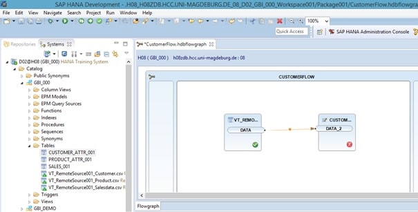
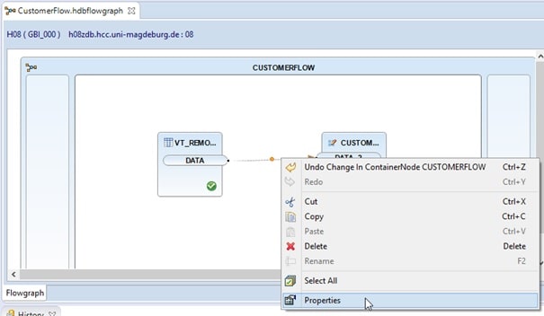
Next, right-click on the connection line and select “Properties”:

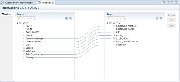
There, perform the field mapping between the virtual table and the data table, by linking the corresponding fields:

Afterwards, save and activate the Flowgraph Model.

8. Execute the Flowgraph Model to load the customer data

In the upper right corner, click on “Open in SQL Editor”:

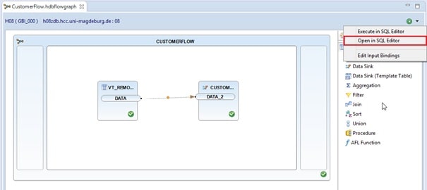
There, remove the leading dot before the package name and run the command:

You can check the successful execution by viewing the content of the table CUSTOMER_ATTR_XXX:

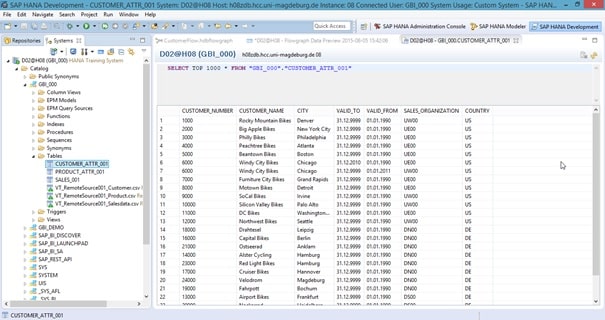
9. Within your project, create a Flowgraph Model for the product data, and load the data. Perform the same steps as you did for the customer data.

Perform the steps 2.6 to 2.8 for the product data.

After performing the steps successfully, the data in table PRODUCT_ATTR_XXX should look as shown in the screenshot below.

10. Within your project, create a Flowgraph Model for the sales data, and load the data. Perform the same steps as you did for the customer data.

Perform the steps 2.6 to 2.8 for the sales data.

After performing the steps successfully, the data in table SALES_XXX should look as shown in the screenshot below.

1. Open the Modeler perspective in the SAP HANA Studio

Step 3: Create an Attribute View for customer data

Window → Open Perspective → Modeler

2. Create a new package to group the views that you will create in the following steps

Navigator View → Content → Right click → New → Package

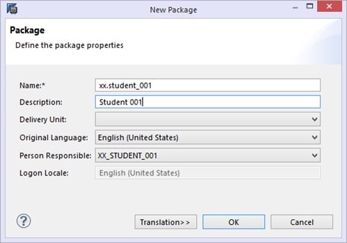
3. In your package, create an attribute view for the customer data

Navigator View → Content → Package xx.student_xxx→ Right click → New → Attribute View…

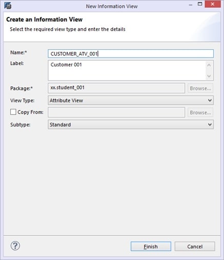
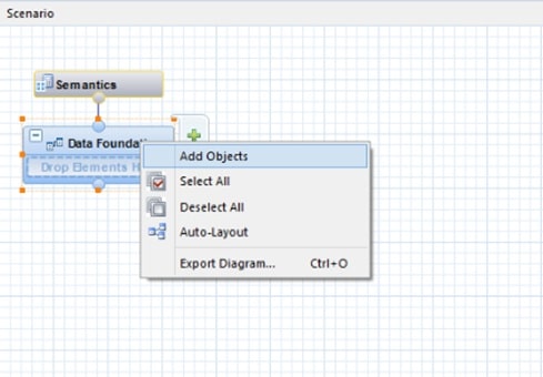
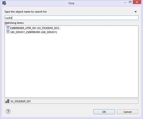
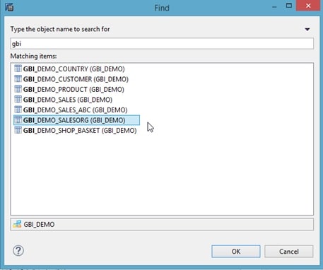
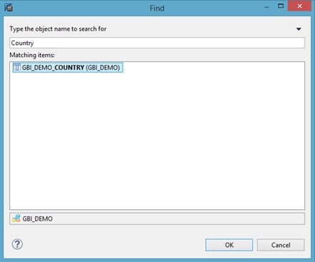
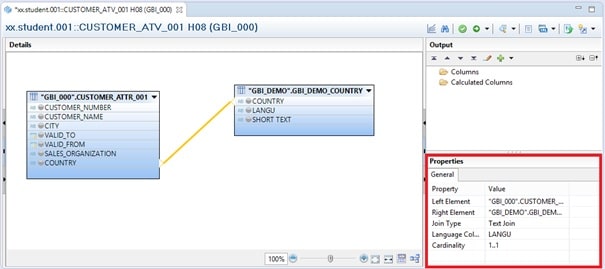
4. Join the table GBI_DEMO_COUNTRY with table CUSTOMER_ATTR_XXX using a text join

Drag & drop the field CUSTOMER_ATTR_XXX.COUNTRY to field GBI_DEMO_COUNTRY.COUNTRY.

Click on the link between the two tables that represents the join. Now you should see the properties of the join on the right.

Adjust the properties as following:

5. Join the table GBI_DEMO_SALESORG with table CUSTOMER_ATTR_XXX using a text join

Drag & drop the field SALES_ORGANIZATION from the customer table to field SALES_ORGANIZATION of table GBI_DEMO_SALESORG.

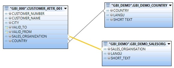
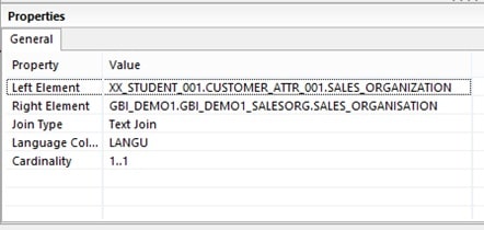
Click on the link between the two tables that represents the join. Now you should see the properties view for the join in the bottom.

Adjust the properties as following:

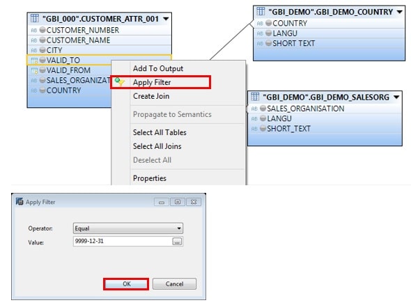
6. The view should show only current customers. For current customers, the valid-to date is equal to 9999-12-31. Add a corresponding filter to your view.

Select the VALID_TO field in the customer table.

Select the option Apply Filter in the context menu if this field.

7. Add all attributes that should be visible in this view to the output structure

Select the table fields that should be visible in the output structure.

Click on Add To Output.

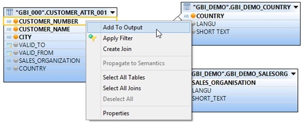
Now the fields should be visible in the output structure.

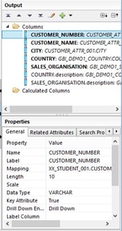
Repeat this for each table field that should be visible in the output structure. Select True for the property Key Attribute to mark an attribute as a key.

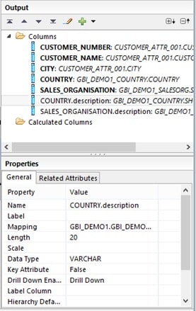
8. Perform the description mapping for the fields COUNTRY and SALES_ORGANISATION in the properties of the output structure

Add the description fields Short Text for both tables to the Output structure.

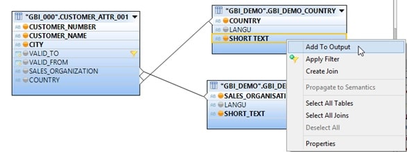
After adding the description fields to the output, click on the output fields of COUNTRY and SALES_ORGANISATION and set the Label Column to Short Text.

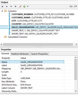
Rename the output fields with the names SHORT_TEXT and SHORT_TEXT_1 to COUNTRY.description and SALES_ORGANISATION.description.

9. Save, validate and activate the Attribute View

Press Save and Validate.

Check the Job Log. In case of an error, the job is highlighted in red.

Press Save and Activate.

Check the Job Log. In case of an error, the job is highlighted in red.

Step 4: Create an Attribute View for product data

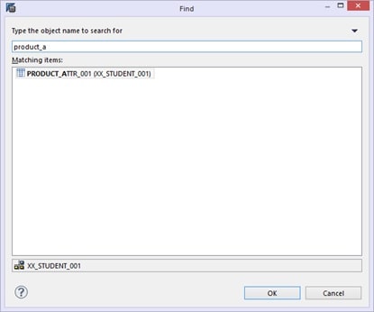
1. Create a new Attribute View for product data in your package

Navigator View → Content → Package xx.student_xxx → Right click → New → Attribute View…

2. Add all relevant attributes to the output structure of the Attribute View

Select the table field that should be visible in the output structure as attribute.
Click on Add To Output.

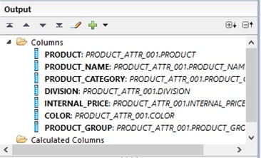
After adding all relevant fields, the output structure should look as following:

3. Save, validate and activate your Attribute View

Press Save and Validate.

Check the Job Log. In case of an error, the job is highlighted in red.

Press Save and Activate.

Check the Job Log. In case of an error, the job is highlighted in red.

1. Create a new Analytic View for the sales data

Step 5: Create an Analytic View

Navigator View → Content → Package xx.student_xxx → Right click → New → Analytic View…

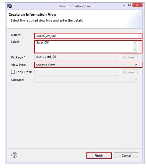
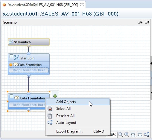
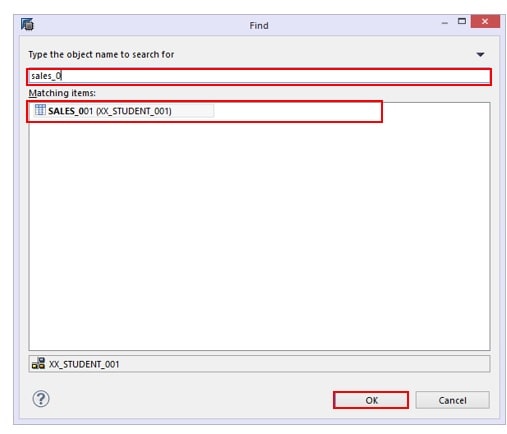
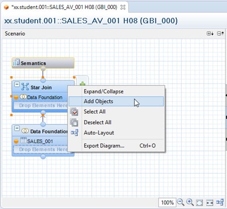
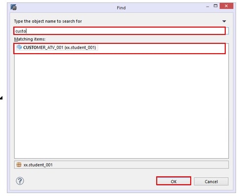
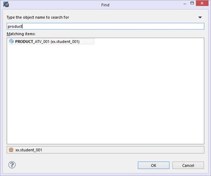
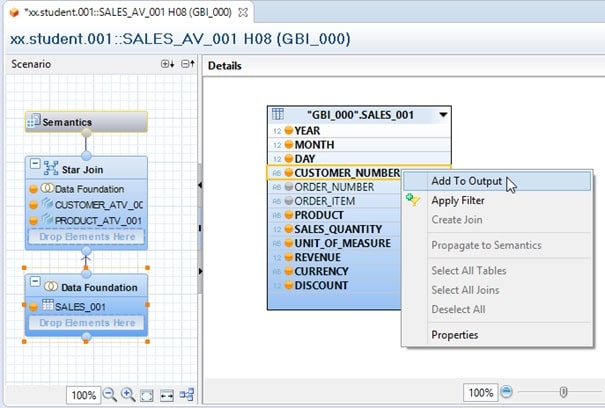
On the Data Foundation component, select the relevant fields of table SALES_XXX and choose Add to Output to add them to the output structure.

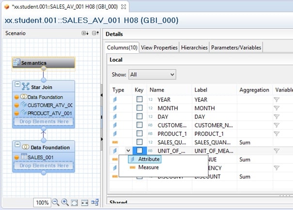
Select the Semantics component to change the type of the output fields.

2. Join the sales table with the product and customer view, using a referential join

Switch to the Star Join component.

Drag & drop field DATAFOUNDATION.CUSTOMER_NUMBER_1 to field CUSTOMER_ATV_XXX.CUSTOMER_NUMBER.

Drag & drop field DATAFOUNDATION.PRODUCT_1 to field
PRODUCT_ATV_XXX.PRODUCT.

3. Add the net sales price as calculated measure to the output structure of your Analytic View

In the output structure of the analytic view, select the folder Calculated Columns and choose New… from the context menu. Enter the details as indicated in the screenshots.

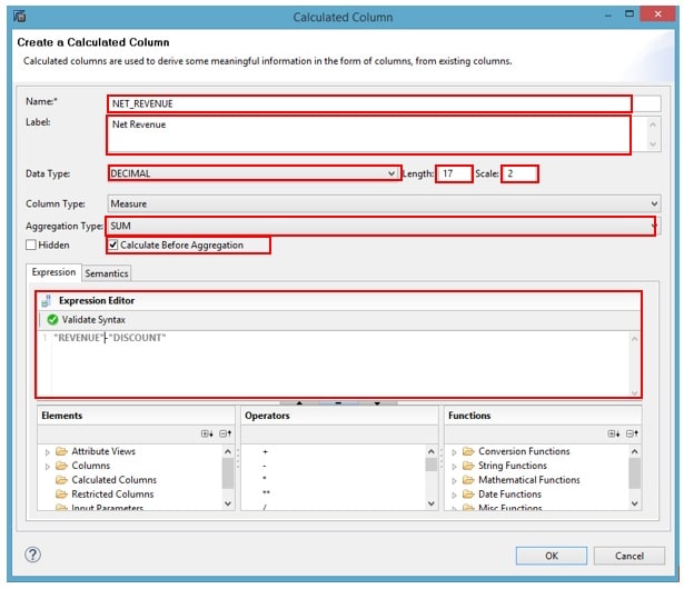
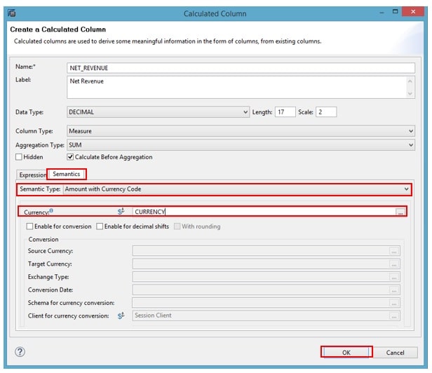
Press OK.

1. Save, validate and activate the Analytic View

Press Save and Validate.

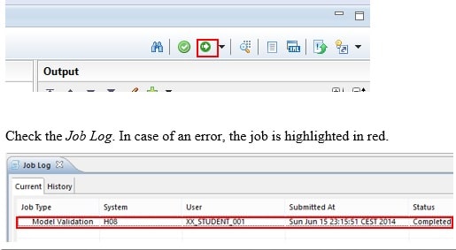
Press Save and Activate.

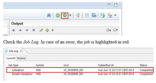
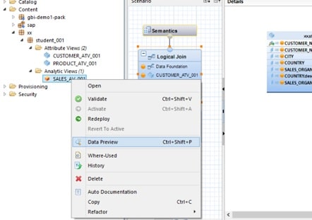
Open the data preview for your analytic view and check the data

Content → xxà GBI_XXX → Right click → Data Preview

Step 6: Analyze the sales data

1. Open SAP Lumira and login with your Credentials

Start Lumira by calling the link provided by your instructor.

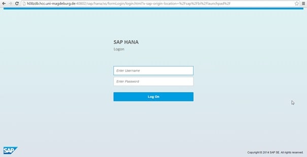
Type in Username and Password and click on Log on.

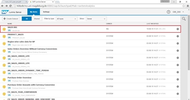
2. Select your Analytic View as basis for your analysis

Click on your Analytic View Sales 001 (SALES_AV_001), which you have created in one of the previous tasks.

3. Analyze the data provided by your Analytic View

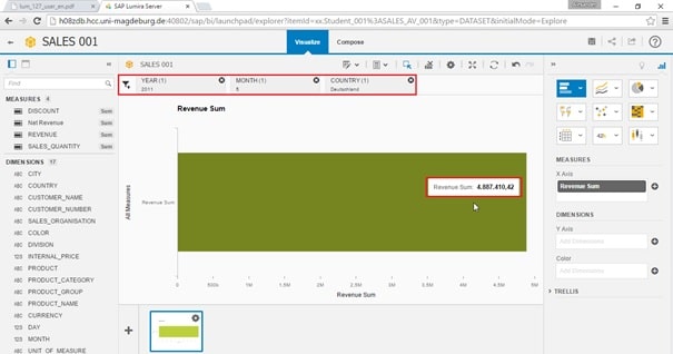
What is the total revenue in Germany in May 2011?

• Select Revenue(SUM) in the Measures section
• Select 2011 as year
• Select 5 as month
• Select Germany as country

The correct answer is: 4.887.410,42 EUR

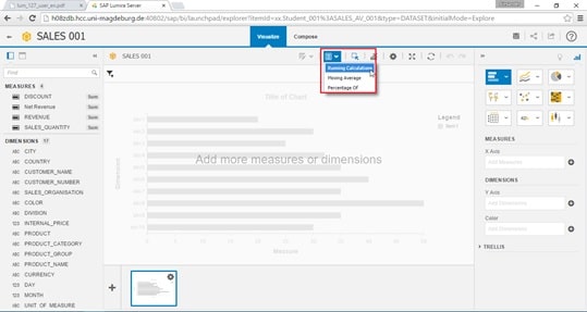
What are the top 3 products by revenue sold in Germany in May 2011?

• Select Revenue(SUM) in the Measures section
• Select 2011 as year
• Select 5 as month
• Select Germany as country
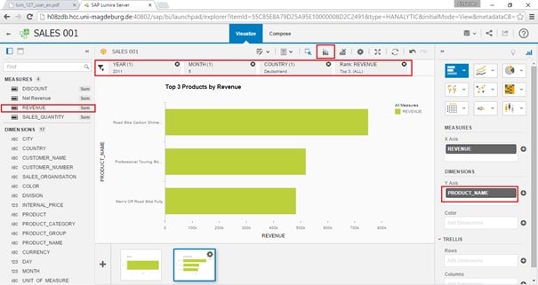
• Select Top 3 and Product_Name (see screenshot)

The screen should look as following: