ENME352-16B Dynamics Assignment
If you obtain advice from others, or use information from any source including the web, these must be acknowledged in your report. Two sample MATLAB codes are provided at the end of the assignment to help you with this assignment. Some steps will be explained in the lectures/tutorials. You are welcome and encouraged to check your answer with me at each starred step.
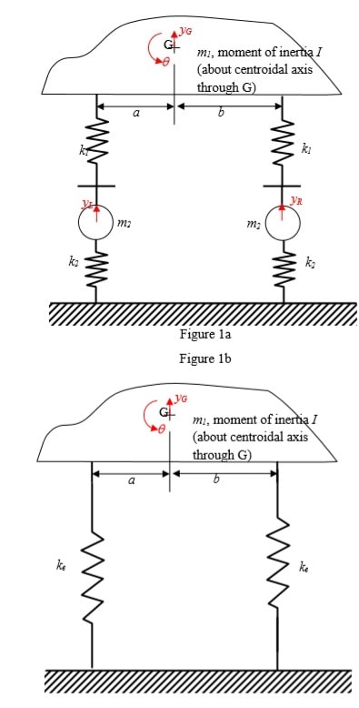
1) The schematics of an electric vehicle is shown in Figure 1a. It is given that k1 = 12500 N/m, k2 = 105 N/m, m1 = 450 kg, m2 = 24 kg, I =96 kgm2, a =0.7 m, b =0.8 m.
a) *First, neglecting the mass of the wheels and taking the equivalent spring stiffness ke at both ends (See Figure 1b) write down the potential and kinetic energy terms in terms of Gy, θ and proceed to derive Lagrange’s equations of motion. You need to first show that as ke = 1/(1/k1+1/ k2).
b) Arrange the equations in matrix form ![]()
c) *Using the MATLAB code given in Appendix 1, find the natural frequencies and modes. You will need to change the definition of elements of the matrices K and M.
d) *Now considering the mass of the wheels, write down the potential and kinetic energy expressions in terms of all four degrees of freedom yL,yR, yG, θ and proceed to derive the equations of motion using Lagrange’s formula.
e) Arrange the equations in matrix form 
f) Modify the MATLAB program given to find the natural frequencies and modes of the vehicle.
g) Obtain the solution to the four dof problem, for the case of m2=0 and compare with results in part (b).
h) Comment on the effect of neglecting the mass of the wheels.

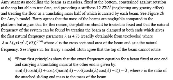
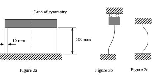
2) Two engineers (fresh graduates) Amy and Barry disagree on how to model a framework that supports a sensitive equipment which needs to be protected against vibration. They are aware that if the framework has a natural frequency close to the frequency of any disturbance, large amplitude oscillations may damage the equipment. The framework consists of two 500 mm long vertical steel (elastic modulus E = 210 GPa, density p= 7800 kg/m3) beams of 24 mm x 10 mm rectangular cross section, connected to a rigid platform of 30 kg mass which supports the instrument of negligible mass. See Figure 2a.

b) Find the first three roots of the above equation using a MATLAB program and solve the problem to compare with Amy’s and Barry’s models and comment on your findings. Consider the vibration of the framework in its plane (see possible modes in Figures 2b and 2c). The bending of the beam will then be about the weaker axis. This is needed to choose the correct breadth and depth in the formula for the second moment of area of a rectangle. A MATLAB code that can be used to find the roots of a frequency equation for a different set of boundary conditions is provided to you. (Appendix 2). You will need to modify this. The statements of the frequency equation that needs to be modified are highlighted.
c) Explain why both agree that the top of the beam cannot rotate.

Appendix 1: Sample MATLAB Code to solve a 2 dof freedom system
{`
%K is the stiffness matrix
%M is the stiffness matrix
% n = number of d.o.f
% w = natural frequency in rad/s
%lamda is the eigenvalue = square of the n.freq given by diagonal elements
% mode = relative displacement =  mode
%ith column in the matrix labelled mode gives the ith mode shape

 n=2;
K=[2.0,-1.0;-1.0,2.0];
M=[1,0;0,1]; [mode,lamda]=eig(K,M);
for i=1:n
w(i)=sqrt(lamda(i,i));
end
w
mode
`}
Appendix 2: Sample MATLAB Code to find the roots of a frequency equation
{`
%this program looks for a change in the sign of the determinant of a
%boundary condition matrix B by trial and error
%It can be used to find the roots of det[B]=0 provided there are no poles -
%that is where the determinant changes sign through a pole clear all
%l1 is the initial trial value for lambda l1=0;
%sl is an initial assignment for the increment in lambda sl=0.1;
%dl is an increment that is continually adjusted to get the results to a
%desired tolerance dl=sl;
% precision/tolerance/accuracy for lambda tol=0.000001;
%set trial lambda l to l1; l=l1;
%set maximum number of trials im to say 5000 to make sure that calculations
%don't continue indefinitely if the step is small or the determinant
%doesn't have any root due to any mistake im=5000;
% j is an integer to count the number of eigenvalues j=0;
%calculate the determinant B using lambda but label it oldetB as it will
%change in the next step. The example given below is for a clamped-simply
%supported beam. The highlighted lines are specific to this boundary
condition and need to be changed for any other case. oldetB=sinh(l)*cos(l)-cosh(l)*sin(l);
% calculation number count i is set to zero initially i=0;
%jm is the maximum number of eigenvalues needed jm=3;  while i< im     i=i+1;     l=l+dl;
detB(i)=sinh(l)*cos(l)-cosh(l)*sin(l);
% the above line is the frequency equation which needs to be changed     trial_lamda(i)=l;

    if sign(oldetB)*sign(detB(i))<0         l=l-dl;
%reduce the increment in lambda to search for the root         dl=dl/2;     else
oldetB=detB(i);     end     if dl< tol         j=j+1;
%lamda is the eigenvalue     lamda(j)=l;     l=l+sl;
%having found one eigenvale now reset the increment to original value     dl=sl;
oldetB=sinh(l)*cos(l)-cosh(l)*sin(l);
% the above line is the frequency equation which needs to be changed     if j>=jm         i=im+1;   end
end end
%the following line displays the results for the roots lambda  lamda
%the following is a plot of the determinant vs trial lamda
figure (1)  plot (trial_lamda,detB)  hold on

  % if the plot doesn't show any poles the roots can be taken as
% correct. Otherwise the program need to be modified to eliminate pole
`}


