MAE256 T2 Sample Assignment

MAE256 T2 – ASSIGNMENT

Answers

Q.1 The descriptive statistics of house sale prices is presented in the Table 1. The output was generated using excel.

Table 1Descriptive statistics of house sale price in thousands of dollars.

From Table 1, it can be seen that the average house sale price in thousands of dollars is $804.88. The median house sale price is $798.95 thousand dollar. The spread of the sale prices can be assessed from the standard deviation which is $137.13 thousand dollar. Therefore, the spread of the data is high. The skewness of the data is very low which is 0.09. Therefore, it can be commented that the data is symmetrical and follows normal distribution. It can also be seen from the difference between mean and media, which are nearly the same considering the size of data. Therefore, the spread of the data is high whereas skewness of the house prices is nearly symmetrical.

Q2. The mean sale price of house is 804.11 and the standard deviation is 137.13. The house price which is one standard deviation away from the mean would be:

µ±σ = [804.11 – 137.13, 804.11 + 137.13] = [666.98, 941.24]. Therefore, as it is known that proportion with one standard deviation away from mean is nearly 68.5%. Hence, 68.5% of the prices are between $668.98 thousand and $941.24 thousand.

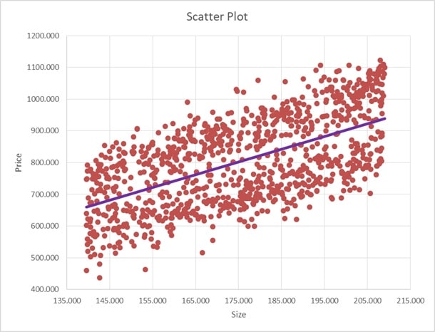
Q.3 The Figure 1 presets the scatter plot of price against the size. It is generated using Excel. It represents size on x-axis and price on y-axis.

Figure 1 Scatter plot between price and size

As it can be seen from the figure that there is a positive relationship between house sale prices and size of the house. It can be interpreted that as the size of house in square meters increases the sale price of house also increases.

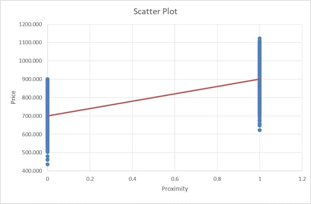
Figure 2 presents the scatter plot between the proximity and price. Proximity is a dummy variable which shows whether the house is located near major business district or not. If house is near a major business district then it takes the value of 1 or 0 otherwise. The proximity is represented on x-axis and sale price is represented on y-axis.

Figure 2 Scatter plot between price and proximity

It can be seen from the above figure, that as the house is more near to the major business district, the price will be higher. Therefore, it can be stated that the proximity of house also affect the sale prices positively. In conclusion, both size and proximity are positively related to the sale prices of house.

Q.4 The linear regression of below stated model is performed using excel,

In the above model, the dependent variable is prices which is regressed with explanatory variables of size, age and proximity. It should be noted that the proximity is dummy variable. The excel output of the above model is represented in Figure 3.

Table 2 Regression Output

Therefore, our estimated model is:

The adjusted R² of the model is 0.866, which is a measure of goodness of fit. The intercept of our model is the base price of the sale price. It is the average price level which is not dependent on any of the explanatory variables. The estimates of slope parameters of size, age and proximity are 3.8901, -0.6016 and 195.8438 respectively. The estimate of slope coefficient of size can be interpreted as the sale price is increased by $3.89 thousand if size increases by 1 square meters, keeping other variables constant. Similarly, if the age of the house is increased by 1 year the sale prices are decreased by $-0.6015 thousand while keeping the effect of size and proximity constant. If the house is near major business district then the proximity variable will take the value of one, therefore, the prices of house which are near business districts are on 195.8438 thousand more as compared to the houses which are not near the business district keeping other factors constant. The results are expected as, the houses with more size and which are near business districts will costs more. The age of house is also very important factor, the more old the age of the house, the prices of house will decrease. It is also important to note that at 5% only size, age and proximity estimates are significant.

Q.5 After adding two more variables of swimming pool and fire place into our previous model, the following model is obtained.

Both the variables that are introduced into the model are dummy variable. Pool variable takes the value of 1 if house has swimming pool or 0 otherwise. Similarly, fireplace takes the value of 1 if house has fireplace or 0 otherwise. The regression was performed using excel, the output is represented in Table 3.

The R² of model before introduction of pool and fireplace variable was 0.8666 and the R² after the introduction of the said variable is 0.8686. As it can be seen that R² of the model is increased very little. Therefore, the introduction of the model did not increase the ‘goodness of fit’ of the model. It is better to also consider the value of adjusted R² as it penalize the model for the introduction of new variables. The adjusted R² before introducing new variable is 0.8662 and after introducing new variable the value of adjusted R² is 0.8679. Therefore, introduction of adding new variable has increased the goodness of fit of the model but with a very modest amount. Nevertheless, the variation explained by the model has increased by introduction of two new variables.

Table 3 Regression output

Q6. After transforming the price and size variables into natural logarithms. The following model is obtained:

The regression was performed using excel and the output is presented in Table 4. The estimated model is following;

Table 4 Regression output

The slope coefficient of log(size), represents the percentage change in percentage change in price due to one percent change in size. Therefore, it can be interpreted as the sale price of houses increased by 84.72% or nearly 85% when there is one percent increase in size of the house. The estimate of  represents the percentage difference in house of sale prices when there is availability of swimming pool in the house keeping size, proximity, age and fireplace constant. Therefore, it can be interpreted as the sale prices of houses with swimming pool availability will be nearly 1.86% more as compared to prices of house which does not have swimming pool.

Q7. Null Hypothesis: H₀: Fireplace does not influence the house prices: H₀:

Alternate hypothesis: H₁ Fireplace influence the house prices: H_a: .

It can be seen from Table 4 that p-value of the estimate of fireplace is 0.08 which is far greater than the 0.01 level of significance. Therefore, at 1% level of significance, cannot reject the null hypothesis as p-value is greater than significance level. Hence, it can be stated that there are no enough evidence to reject the claim that fireplace does not influence the house prices. However, at 10% level of significance, the p-value is smaller than 0.10, therefore, we can state that there are enough evidences to reject the null hypothesis. Hence, it can be stated at 10% level of significance that fireplace does influence the sale prices of house.

Q.8 Null Hypothesis: all the variables in the model are not significant.

Alternate hypothesis: at least one coefficient is different from zero.

According to the output generated in Table 4, it can be seen that p-value of F statistic is given by 0 which is lower than the 0.05 level of significance. Hence, there are enough evidences to reject the null hypothesis. Therefore, it can be concluded that the variables are jointly significant. Hence at least one variable from size, proximity, age, pool and fireplace affects the sale prices of house.