European Carbon Dioxide Emissions for Passenger Cars Sample Assignment

European Carbon Dioxide Emissions for Passenger Cars

Data Preprocessing

Data preprocessing included observing the datasets and analyzing categorical variables using table () function in r to check the consistency of the grouping criteria. Variables which are intended to be used in the model were highly focused, hence assuming variables like car make which has a lot of categories, and hence they may not be of much help in the model. I checked fuel type and technology type, which are denoted as Fueltype and Technoltype in the dataset respectively. These variables had a mixture of lower and upper cases denoting the variables, which led to similar categories of the variables. To dissolve this data compatibility issues, I used the letter case package to standardize the cases. Within this package, there are several functions which allow transformation of string variables in R. some of these functions include str_capitalize and str_to_title. The former is used to change strings into either lower or upper case. The latter function only transforms the strings into title case which is the upper case. There are several other within the same function, just to allow transformations within string variables(Eberly, 2007; Faraway, 2002).

Transforming Fuel Type variable

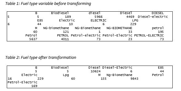
Formally, the fuel type categorical variable had 20 groups which were as a result of duplicated groups. The variable is a factor variable hence the need to transform into character to allow the functionality lettercase package function and then transform back to factor using as.character() and as.factor() functions respectively. After the transformation, the categories reduced to 11 groups.

Transforming Technology type variable

Before the technology type variable’s compatibility issues were handled using the str_capitalize variable, there were 25 categories. After the transformation, the categories reduced to 19.

Transforming Innovative Technologies variable (ITReduction)

This variable has 5 categories amongst which 4 represent car models with innovative technologies to reduce CO2 emissions. From this variable, I created a dummy variable ITReduction_Dummy with 1 denoting whether a car has the innovative technology to reduce CO2 emission and 0 otherwise(Fox & Weisberg, 2002).

Table 3: ITReduction tabled categories

Table 4: Innovative Technology dummy variable

Years before and after Volkswagen CO2 emission scandal

It was indicated that the years variable within the dataset represented before and after the time of the Volkswagen’s CO2 emission scandal. This can be a good predictor in modelling to check the effect of the scandal on the manufacturer’s decisions. Therefore, I created a dummy variable with 1 representing post-time and 0 representing the time before the scandal.

The table above shows that around 45.8% of the cars were obtained from the time before the Volkswagen scandal, while 54.2% posted the event. There was no entry with a missing value on the year variable.

Splitting the dataset

From the data description, it has been mentioned that values of CO2 emission variable have been

removed for the purposes of prediction. Therefore, I used this criterion to split the data into train and test datasets, which consisted of 66.7% and 33.3% respectively of the entire data.

Exploratory Data Analysis

Exploratory data analysis is dependent on the type of model to be used for the data. For instance, linear regression assumes that there are linear relationships between the response variable and the predictors. Therefore, the relationships and correlations can be assessed in the exploratory data analysis stage. Secondly, the response variable is assumed to be approximately normally distributed. After checking for normality either by using the histogram or statistical tests, methods like the transformation of the variable can be used reduce the effect of extreme values. After plotting a histogram, it was observed that there were extreme values was affecting the distribution. The plot can be seen in the figure below.

The response variable

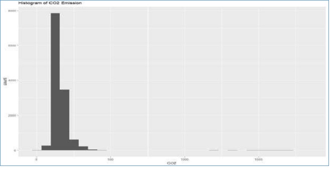
Figure 1: Histogram of CO2 Emissions

Log transformation was conducted to reduce the effect of the extreme values observed in figure

1. Below is the histogram of the natural log of CO2 emissions(Ghasemi & Zahediasl, 2012).

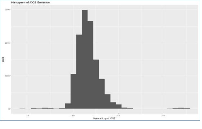
Figure 2: Histogram of Natural Log of CO2

Comparing to the histogram of CO2 emissions and natural log of CO2, the latter shows reduced the effect of extreme values. Therefore, the response variable will be used as log-transformed of CO2 emissions.

The relationship between a Response variable and Predictors

Years before and after Volkswagen scandal

Information 46.4% of the cars in the training dataset were gathered before the CO2 emission scandal happened, while 53.6% were obtained after the scandal. The median log of CO2 emission was higher for the before scandal group compared to the after VW scandal group(Zou, Tuncali, & Silverman, 2003).

$Before

Min. 1st Qu. Median Mean 3rd Qu. Max.

1.447 2.111 2.179 2.195 2.255 3.227

$After

Min. 1st Qu. Median Mean 3rd Qu. Max.

1.556 2.072 2.134 2.147 2.210 3.262

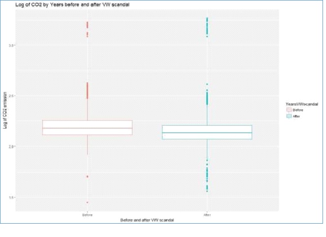
Figure 3: Boxplots of Years of VW scandal dummy by the log of CO2 emission

Figure 3 above shows that the amounts of CO emission reduced after the Volkswagen CO2 emission scandal based on the median statistics. More cars had lower CO2 emissions after the scandal compared to the emissions before the event. The logs of CO2 emissions for both groups are approximately normal. Therefore, the years before and after Volkswagen CO2 emission scandal dummy variable can be a good predictor of CO2 emission levels(Eberly, 2007).

Innovative Reduction Technology

Approximately 97.6% of the cars in the training dataset did not have innovative reduction technology while only 2.4% had the technology installed on the engines.

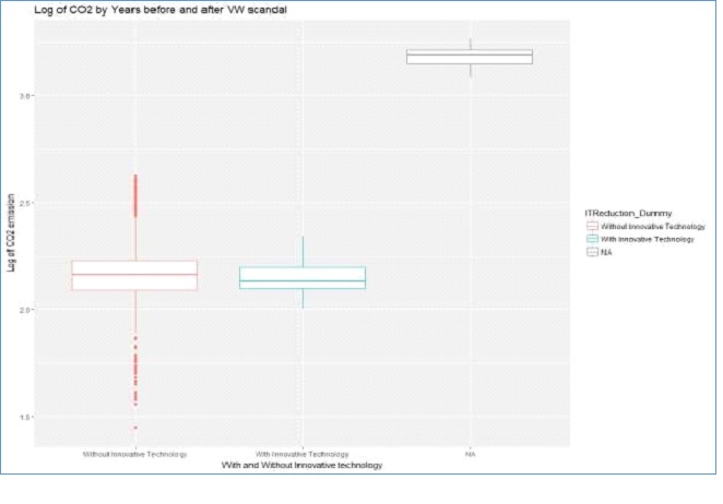
Figure 4: Boxplots of Innovative Technology by Log of CO2 emission

According to figure 4 above, cars without innovative reduction technology had higher CO2 emissions on average compared to those with the technology. Also, cars whose information on Innovative Technology were missing seems to have very high emissions of CO2 compared to the others.

Year

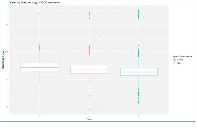
Figure 5: Boxplots of Year by Log of CO2 emission

Figure 5 indicates that CO2 emission has been reducing from the first year to the third year, which depicts that the Volkswagen scandal might not have affected the manufacturers’ decisions.

The weight of the car (Mass)

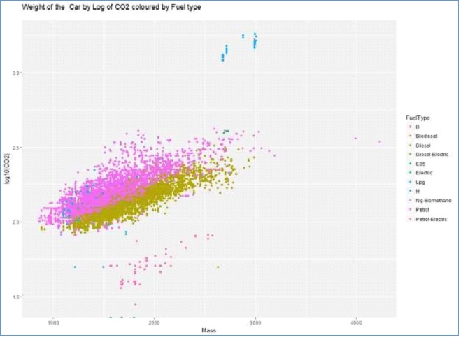
Figure 6: Scatter plot of Mass by Log of CO2

Figure 6 indicates that there is a positive linear relationship between the weight of a car and their CO2 emission. In addition, it also depicts the possible interaction between fuel type and mass in predicting the CO2 emission of a car. From this information, we can create dummy variables for petrol and diesel fuel types to allow interaction terms. We choose petrol and diesel because these are the main fuel types in the dataset(Zou et al., 2003).

Engine Size

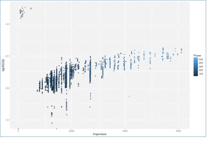
Figure 7: Engine Size by Log of CO2 Emission

Figure 7 above shows that there is a positive linear relationship between engine size and CO2

emissions. In addition, the power of the car also increases with increase in the engine size, which is a clear indication that is a positive relationship between the power of a car and CO2 emission.

Power

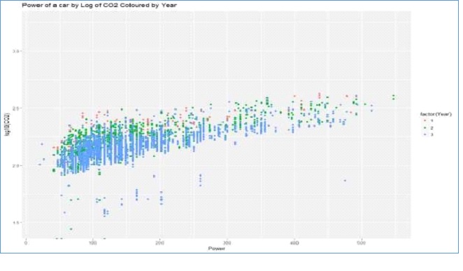
Figure 8: Scatter plot of Power of a car Log of CO2

Figure 8 above shows that there is a positive linear relationship between the power of a car and levels of CO2 emission. The levels of CO2 emission have been reducing significantly from the first year through the third and the trend is consistent despite the power of the car.

Model

I chose a linear model to predict CO2 emissions because the response variable is continuous. Since

there are multiple predictors, I will use multiple linear regression and use the set of predictors to build a prediction model. Further, I analyzed the response variable which is the CO2 emissions and found that there were extreme values. To reduce their effect in the analysis, I decided to introduce natural log for transformation. After transformation, the distribution of the variable changed to approximately normal. After conducting exploratory data analysis, several covariates were found to have a linear relationship with a log of CO2 emission. Their variables include mass, engine size and power of the car. Further, there are several other categorical variables whose categories seem to have different measures of variation and central tendency, hence the possibility of being significant predictors of CO2 emission. Their categorical variables include innovative emission reduction technology and years before & after Volkswagen’s scandal. There are several possible interactions such as fuel type and weight of a car.

Multiple Linear Regression Model

After developing a series of models, it was found that seven predictors could be used in predicting the amount of CO2 a particular car could emit. These variables include Mass, Engine Size, Power, and dummy variable on time before and after Volkswagen’s CO2 emission scandal, the presence of innovative technology on emissions and dummy variables of petrol and diesel use. Using this set of variable, the model was found to be statistically significant with a p-value <0.0001 and adjusted R-squared value of 70.24. This indicates that having all these information, an individual can approximate the amount of CO2 a passenger car could emit. Below is the Model’s R output.

The model can be written as follows

𝑙𝑜𝑔𝐶𝑂2 = 1.727 + 0.000152𝑀𝑎𝑠𝑠 + 0.000049𝐸𝑛𝑔𝑖𝑛𝑒𝑆𝑖𝑧𝑒 + 0.000057𝑃𝑜𝑤𝑒𝑟

− 0.038𝐴𝑓𝑡𝑒𝑟𝑉𝑊𝑆𝑐𝑎𝑛𝑑𝑎𝑙 − 0.0282𝐼𝑛𝑛𝑜𝑣𝑎𝑡𝑖𝑣𝑒𝑇𝑒𝑐ℎ + 0.152𝑃𝑒𝑡𝑟𝑜𝑙 + 0.0671𝐷𝑖𝑒𝑠𝑒𝑙

Model summary

According to the above model, the CO2 emission of any particular car would be approximately 53.33grams/ kilometres assuming that all other factors are held constant. The weight of the car has a positive linear correlation with the amount of CO2 a car emits. It is a significant predictor in the model with p-value <0.0001. Increasing the weight of a car by 1 kilogram, the amount of CO2 emitted increases by 1.00035g/km with other factors being held constant.

The size of Engine of a car is also a significant predictor of the amount of CO2 is emitted(Krzywinski & Altman, 2013). If the size of the engine is increased by 1 cubic centimetres, the amount of CO2 emitted increases by 1.000113 grams/ kilometre. Similarly, as the engine power increases so does the amount of CO2 emitted. Therefore, increasing the power by 1KW, the emission levels increases by 1.00013grams/ kilometre.

Comparing the amount of emission for cars whose information was gathered before and after the Volkswagen’s CO2 emission scandal happened, we find that cars manufactured post the event emitted lower amounts by approximately 1.0914grams/km(Sainani, 2013). Therefore, we can conclude that the scandal led to a positive effect on ensuring that manufacturers produced cars which were more environmentally friendly.

The use of the technological device to reduce the amounts of CO2 emission has significantly succeeded. According to our model, we can conclude that cars which had an innovative technological device to reduce emission were producing fewer levels of CO2 compared to the others. Therefore, a car having the device was associated with low amounts of CO2 emission by approximately 1.0671grams/km.

The variable which was a good predictor of levels of emissions was the fuel type. This was presented as a categorical variable with 11 groups. Among the 11 groups, only two had significant proportions (Diesel – 49.9719% and Petrol – 46.67%), hence the decision to create dummy variables for diesel and petrol. Within the model, the two dummy variables were statistically significant with p-values less than 0.0001. Comparing cars which were using Diesel against the others, the CO2 emissions were high by approximately 1.167grams/ kilometre. Similarly, passenger cars using petrol were emitting higher levels of CO2 on average by approximately 1.45grams/ kilometre(Eberly, 2007).

Potential Limitations of the model

The multiple linear models have several limitations, which might affect the prediction procedure. These limitations are defined below.

1. The model does not allow used a lot of predictors. For instance, we could not include a categorical variable such as the make of the car which has a lot of categories. This is because as the number of categories increase in the categories, the number of variables increases. Many predictors increase the complexity of interpreting the model. They also reduce the power of the model by decreasing the R-squared value(Aiken, West, & Pitts, 2003).
2. The model is sensitive to outliers, hence the need to handle them before fitting the model. For instance, we had to transform the response variable because it had outliers before fitting the model.
3. The model only checks the relationship between the mean of CO2 emission and the predictors, hence the availability of prediction errors.
4. The model is limited to linear relationships between the response variable and the predictors. This is why it is important to conduct exploratory data analysis as a step of building the model. Due to this limitation, it is not possible to include predictors which show other forms of relationships(Kamer-Ainur & Marioara, 2007).

Prediction

The summary statistics of the predicted CO2 emission and the standard errors are shown below

References

Aiken, L. S., West, S. G., & Pitts, S. C. (2003). Multiple Linear Regression. Handbook of Psychology, 481– 507. https://doi.org/10.1051/eas/1466005

Eberly, L. E. (2007). Multiple linear regression. Methods in Molecular Biology (Clifton, N.J.), 404, 165– 187. https://doi.org/10.1007/978-1-59745-530-5_9

Faraway, J. J. (2002). Practical Regression and Anova using R. Reproduction, 21(July), 212.

https://doi.org/10.1016/0360-1315(91)90006-D

Fox, J., & Weisberg, S. (2002). An {`{R}`} Companion to Applied Regression. Sage Publications, (June), 2–3. https://doi.org/10.1177/0049124105277200

Ghasemi, A., & Zahediasl, S. (2012). Normality tests for statistical analysis: A guide for non-statisticians.

International Journal of Endocrinology and Metabolism, 10(2), 486–489. https://doi.org/10.5812/ijem.3505

Kamer-Ainur, A., & Marioara, M. (2007). Errors and Limitations Associated with Regression and Correlation Analysis. Statistics and Economic Informatics, 710–712. Retrieved from http://steconomiceuoradea.ro/anale/volume/2007/v2-statistics-and-economic-informatics/1.pdf

Krzywinski, M., & Altman, N. (2013). Points of significance: Significance, P values and t-tests. Nature Methods. https://doi.org/10.1038/nmeth.2698

Sainani, K. L. (2013). Understanding linear regression. PM and R, 5(12), 1063–1068.

https://doi.org/10.1016/j.pmrj.2013.10.002

Zou, K. H., Tuncali, K., & Silverman, S. G. (2003). Correlation and Simple Linear Regression. Radiology, 227(3), 617–628. https://doi.org/10.1148/radiol.2273011499