ECON 311 IT assignment in Econometrics

Question 1: Estimate model 1, interpret the significance of the estimated coefficients, the overall validity of the model and the coefficient of determination.

Answer.

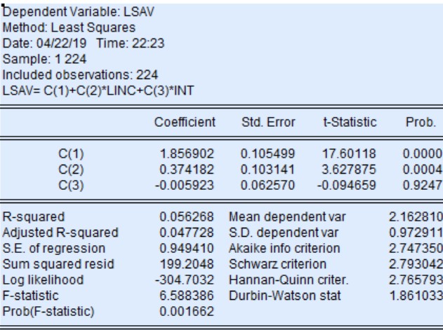
We have estimated the model

where,, and are the logarithm of saving, income and interest rate respectively.

C(1) denotes the level of savings if both income and interest rate are zero.

C(2) denotes the coefficient of logarithm of income. It signifies that 1% increase in income results in 0.37% increase in saving holding other things constant.

C(3) denotes the coefficient of interest rate. It signifies that 1% increase in interest rate causes savings to decline by 0.006 % holding other things constant.

R-square is also known as coefficient of determination. The value of r square is 0.056. It implies that 5.6% of variation in the dependent variable is explained by independent variables i.e. income and interest rate.

Question 2: Report the histogram of the residuals series obtained from model 1, tests whether the residuals series are normally distributed or not?

Answer.

Histogram of the residual series obtained from Model 1.

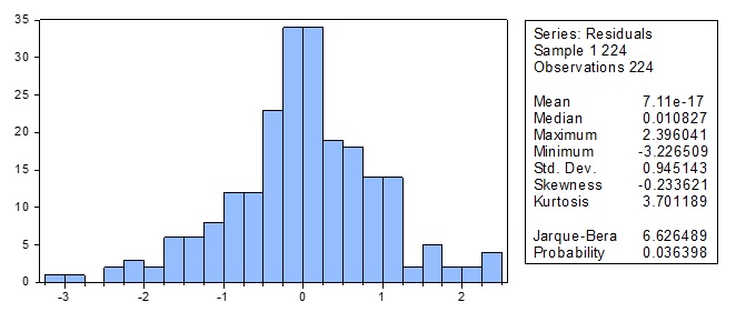
To check whether residuals are normally distributed or not, Jarque -Bera test is used. The null hypothesis of the JB test is that residuals are normally distributed. For the residuals of model 1, we reject the null hypothesis of normal distribution at the 5% level but not at the 1% significance level. Thus, residuals are normally distributed at 1% significance level.

Question 3: Using the Eviews test the homoscedasticity assumption of the residuals using the Breush-Pagan-Goldfrey and White tests.

Report and interpret the results and tests the hypothesis of homoscedasticity against heteroscedasticity.

Answer.

Results of Heteroskedasticity Test using Breush-Pagan-Goldfrey Test

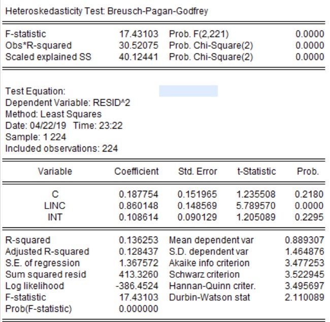
The null hypothesis of the BP test is that residuals are homoscedastic. As p value of the F-statistics is less than 0.05, we reject the null hypothesis that residuals are homoscedastic.

Results of Heteroskedasticity Test using White Test

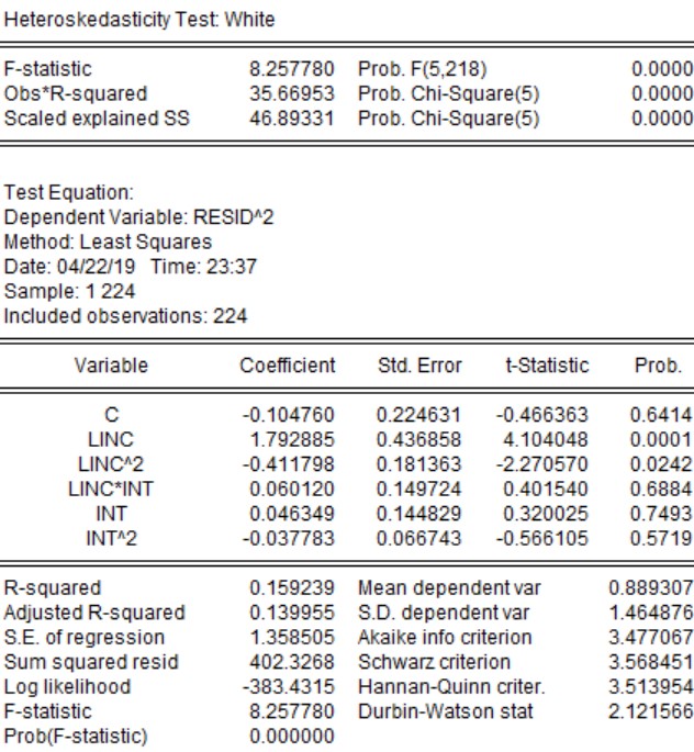
The null hypothesis of the White test is that residuals are homoscedastic. As p value of the F-statistics is less than 0.05, we reject the null hypothesis that residuals are homoscedastic.

Part II

Question 1: for this data we suspect two kinds of heteroscedasticity:

1. V(ε)=σ² |int_i | (heteroscedasticity case1)
2. V(ε)=σ² linc_i(heteroscedasticity case2)
3. For each case 1 and 2 write the weighted model to be used to remove the heteroscedasticity.

Answer.

Case 1

We have heteroscedasticity of following type:

V(ε)=σ² |int_i | (heteroscedasticity case1)

To remove the heteroscedasticity, we will use the following weights: w_i=1/i√int_i

Multiply initial equation with weights w_i*lsav_i=w_i*β₀+β₁ (w_i*linc_i)+β₂ (w_i*int_i)+w_i*ε_i

Weighted model in case 1 will be lsavs_i=β'₀+β'₁ lincs_i+β'₂ ints_i+ ε'_i

Case 2

We have heteroscedasticity of following type:

V(ε)=σ² linc_i (heteroscedasticity case1)

To remove the heteroscedasticity, we will use the following weights: w_i=1/i√linc_i

Multiply initial equation with weights w_i*lsav_i=w_i*β₀+β₁ (w_i*linc_i)+β₂ (w_i*int_i)+w_i*ε_i

Weighted model in case 2 will be lsavs'_i=β''₀+β''₁ lincs'_i+β''₂ ints'_i+ε''_i

Question 2: For each case (case 1 and case 2) estimate the weighted model. To do this you need to create a new variable.

For case one Call them x1, lsavs1, lincs1 and ints1 for the intercept c and the variables lsav, linc and int, respectively. These variables are the weighted new variables of the intercept and the other explanatory variables lsav, linc and int.

For case two Call them x2, lsavs2, lincs2 and ints2.

1. Estimate the weighted model case 1
2. Estimate the weighted model case 2

Interpret the results of the previous two models and determine which of the two cases resolve the problem of heteroscedasticity?

Answer.

Case I

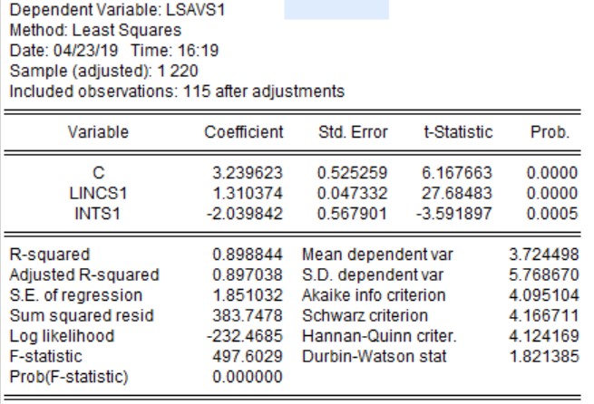
We have estimated the model lsavs_i=β'₀+β'₁ lincs_i+β'₂ ints_i+ε'_i

C(1) denotes the level of savings if both income and interest rate are zero.

C(2) denotes the coefficient of logarithm of income. It signifies that 1% increase in income results in 1.31% increase in saving holding other things constant.

C(3) denotes the coefficient of interest rate. It signifies that 1% increase in interest rate causes savings to decline by 2% holding other things constant.

In case I, the coefficient of determination i.e. r-square improves significantly. 89% of variation in dependent variable is now explained by independent variable.

Case II

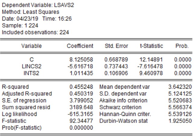
We have estimated the model lsavs'_i=β''₀+β''₁ lincs'_i+β''₂ ints'_i+ε''_i

C(1) denotes the level of savings if both income and interest rate are zero.

C(2) denotes the coefficient of logarithm of income. It signifies that 1% increase in income results in 5.6% decline in saving holding other things constant. This is not a correct relationship.

C(3) denotes the coefficient of interest rate. It signifies that 1% increase in interest rate causes savings to increase by 1% holding other things constant. This is not a correct relationship.

In case II, the coefficient of determination i.e. r-square also improved. 45% of variation in dependent variable is now explained by independent variable. However, this model doesn’t show correct relationship between the variables

Question 3: Report the results of the Breusch-Pagan-Goldfrey and white tests of heteroscedasticity for each case.

Answer.

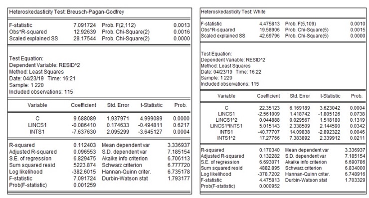
Case I

The null hypothesis of both BP and White test is that residuals are homoscedastic. In case of BP test, we reject the null hypothesis of homoscedasticity at the 5% level but not at the 1% significance level. In case of white test, we reject the null hypothesis of homoscedasticity at the 1% significance level.

Case II

The null hypothesis of both BP and White test is that residuals are homoscedastic. In both cases, we reject the null hypothesis of homoscedasticity at the 1% significance level.

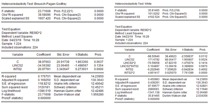
In both case I and II, the problem of heteroscedasticity still persists despite transforming the equations.

Question 4: Report the histogram of each weighted model that you have estimated and interpret the result.

Answer.

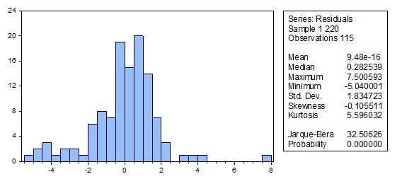
Case I

To check whether residuals are normally distributed or not, Jarque -Bera test is used. The null hypothesis of the JB test is that residuals are normally distributed. For the residuals of case I, we reject the hypothesis of normal distribution at the 1% significance level.

Case II

To check whether residuals are normally distributed or not, Jarque -Bera test is used. The null hypothesis of the JB test is that residuals are normally distributed. For the residuals of case II, we reject the hypothesis of normal distribution at the 1% significance level.

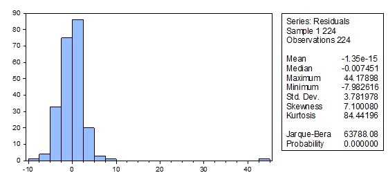
In both case I and II, residuals are not normally distributed.

Question 5: what is your conclusion?

Answer. We can conclude the following based on above results:

• In both models, residuals are not normally distributed.
• In both cases, problem of heteroscedasticity still persists.

Thus, despite transforming the equations to weighted least square the problem of heteroscedasticity persists. We need to use other methods to solve this problem or the heteroscedasticity is not of the form assumed above.