Microeconomics Assignment Help With Theory Of Production
Meaning of production
Production is an economic activity that makes goods available for consumption. Production at times is also defined as all economic activities minus consumption. It is the process of creating goods or services using various available resources.
Production function and Factors of production
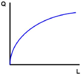
Production function shows the relationship between the quantity of a good/service produced (output) and the factors or resources (inputs) used. The inputs used for producing these goods and services are called factors of production.
- Variable factor of Production: A variable factor of production is one whose input level can be varied in the short run. Raw material inputs are a variable factor and unskilled labour is usually thought of as a variable factor.
- Fixed factor of production: A fixed factor of production is one whose input level cannot be varied in the short run. Capital is usually a fixed factor. Capital refers to resources such as buildings and machinery etc.
Thus production generally represented as a function of capital and labour.
Q = F (K, L)


Production Possibilities frontier
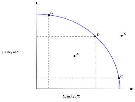
Production possibilities frontier (PPF) curve represents all combinations of goods and services that can be produced using the available goods and resources. The PPF curve is also called Transformation curve. This curve shows the maximum quantity of goods/services that can be produced given the availability of the factors of production. As can be seen from the figure below point X lies beyond the PPF curve and thus the output level of X can't be reached. Similarly point A lies below the PPF curve which means that the production is below the efficient level. Points B, C and D are different combinations of quantity produced of Good X and Good Y. At all these points the resources or inputs are efficiently utilised.

Isoquants
Isoquants are those combination of inputs or factors of production which provides an equal or same quantity of output. Isoquant curves are also called Equal product or iso product curve. For a production function which denotes isoquant:
Q=F(L,K),
Q is fixed level of production
L = labour and K = Capital are variable
The table below shows different combinations of labour and capital required to produce 100 shirts
| Labour (L) | Capital (K) | Output (Shirts) |
| 10 | 90 | 100 |
| 20 | 60 | 100 |
| 30 | 40 | 100 |
| 40 | 30 | 100 |
| 50 | 20 | 100 |
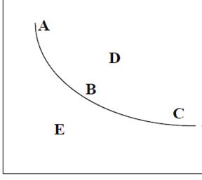
Different resources/ inputs are required for production of goods. Same number of outputs can be produced using different input combinations. Isoquant is the combination of all such combination of inputs which produces same output. Thus we have an isoquant curve for every level of output. Since the quantity produced will remain unchanged on an isoquant, the producer is indifferent for different input combinations. In the figure below the producer will be indifferent on points A, B and C since they are on the same isoquant. Also he cannot move to D without increasing both the inputs and would not produce at E due to inefficiency.

Similar to Indifference curve as one move to the right of the isoquant, one reaches a higher level of production.
Returns to a factor
In the short run the output can be increased for a production function by increasing the amount of the variable factor, usually taken to be labour. Thus the responsive change in the output due to a change in the variable input keeping all other things constant is called returns to a factor.
Law of variable proportions
In short run the output of goods and services is increased by introducing additional variable factor to the production process to a said quantity of fixed factors.
Law of variable proportions outlines the various possible output scenarios due to the change in the proportions of fixed and variable factors used for production. If we increase the number of a factor (labour) keeping all other factors fixed (capital), then the proportion between the fixed and variable factors is changed.
The law of variable proportions implies that as we keep on adding the variable factor of production the marginal product of that factor keeps on decreasing progressively. Thus after a point every additional unit of factor added will result in a smaller increase in output.
The law of variable proportion is also known as law of diminishing marginal returns or law of diminishing returns.
The law has several assumptions as below:
- one input is variable while others are fixed in the short run
- all units of the variable input are same and have equal efficiency
- no change in production technology
- factors of production like land and labour can be used in different proportions
Take for instance, hiring additional employees (a variable resource) to work at a factory will initially increase output but eventually it will become more and more difficult to generate additional output from the fixed resources (due to plant size and equipment limitations) and thus the total output will increase at a decreasing rate and ultimately will start decreasing
To further understand this let us consider an example of production of shirts in a factory
Refer to the table below:
| Labour (workers/day) | Total Product (shirts per day) | Marginal product (shirts per additional worker) | Average Product (shirts per worker) |
| 1 | 2 | - | 2.00 |
| 2 | 5 | 3 | 2.50 |
| 3 | 9 | 4 | 3.00 |
| 4 | 12 | 3 | 3.00 |
| 5 | 14 | 2 | 2.80 |
| 6 | 15 | 1 | 2.50 |
| 7 | 15 | 0 | 2.14 |
| 8 | 14 | -1 | 1.75 |
The numbers in the above table shows that as additional number of workers are put on work the total production of shirts increases.
| Total product is the maximum output that a given quantity of input can produce |
Marginal product is the increase in total output due to an increase in a unit of input (labour) with all other inputs remaining constant. |
Average product is the average quantity of shirts produced by each worker. This tells us how productive workers are on an average. |
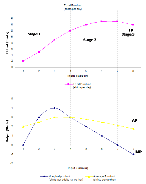
As we can see from the above table, marginal product at first increases and then starts decreasing. Average product also similarly first increases and then starts decreasing. The relationship between these 3 product concepts and input can be further explained using the three product curves below

In the figure above the input (labour) is shown on x axis while the output (shirts) are shown on the y axis. As we can see from the figure upto three input units the production increases at increasing rate and thus marginal product (MP) is highest. After this MP curve starts declining and intersects average product (AP) curve. At this point AP is highest and after this AP also starts to decline. At 7 input units the total product is maximum and MP is zero. Thereafter TP starts decreasing leading to negative marginal product
The three stages of production as shown above in the figure above can be summarised as follows:
| Stages | Total Product(TP) | Marginal Product (MP) | Average product (AP) |
| Stage 1 | Increase at increasing rate and than at diminishing rate | Initially increases and reaches the maximum point, thereafter starts decreasing | Increases and reaches its maximum. At this stage AP=MP |
| Stage 2 | Continues to increase and reaches its maximum | Continues to decrease and reaches to zero | Starts to diminish. Remains above the MP curve |
| Stage 3 | Starts decreasing | Moves to negative territory | Continues to decrease but always remains above zero |
Relationship between MP and TP
From the above table and figure we can identify the following relationship between MP and TP
- As long as MP is increasing, TP will increase at increasing rate
- When MP starts diminishing, TP will increase but at a decreasing rate
- When MP is zero, TP remains unchanged and is at its maximum. Thus
At MP=0, TP is maximum
- When MP is negative, TP starts decreasing
Relationship between MP and AP
Similar to the relationship between MP and TP, we can also observe the relationship between MP and AP from the table and figure discussed above
- AP increases till MP>AP
- AP decreases when MP<AP
- AP is maximum when AP=MP
- MP can be zero or negative, but AP continues to be positive always
Returns to scale
In the long run output of goods can be increased by increasing all the factors (i.e. both labour and capital). In the long run all factors are variable, thus the responsive change in the output due to proportional change in the size or scale of inputs or factors of production is called returns to scale.
For instance, if the initial production function is as below:
P= f(K, L)
and the factors of production K and L are increased in same proportion, than the new production function will be:
P1= f(aK,aL)
- Constant returns to scale: When P1 increase in the same proportion as the factors of production it is called constant returns to scale. Thus in this case
P1/P = a
- Decreasing returns to scale: When P1 increases less than the proportionate increase in the factors it is called decreasing returns to scale, i.e.
P1/P < a
- Increasing returns to scale: if P1 increases more than the proportionate increase in the factors of production it is called increasing returns to scale, i.e.
P1/P > a
The three stages of returns to scale are also explained with the help of the table below:
| Labour | Capital | % increase in inputs | Total Product | % increase in total product | Returns to scale |
| 1 | 2 | - | 10 | - | |
| 2 | 4 | 100% | 30 | 200% | Increasing |
| 3 | 6 | 50% | 60 | 100% | Increasing |
| 4 | 8 | 33% | 80 | 33% | Constant |
| 5 | 10 | 25% | 100 | 25% | Constant |
| 6 | 12 | 20% | 110 | 10% | Decreasing |
7 | 14 | 17% | 120 | 9% | Decreasing |
| 8 | 16 | 14% | 125 | 4% | Decreasing |
| constant returns to scale if (for any constant a greater than or equal to 0) F(aK, aL) = aF(K,L) |
| increasing returns to scale if (for any constant a greater than 1) F(aK, aL) > aF(K,L) |
decreasing returns to scale if (for any constant a greater than 1) |
Microeconomics Assignment Help | Microeconomics Help | Theory Of Production | Microeconomics Theories | Theory Of Production | Production Efficiency | Production Theory | Average Product | Theory Production | Online tutoring


