Microeconomics - Competition and Market Structures, Economics Study
What is Microeconomics?
Microeconomics is the branch of economics that analyzes the market behavior of individual consumers and firms in an attempt to understand the decision-making process of industries/firms and households. It is concerned with the interaction between individual buyers and sellers and the factors that influence the choices made by buyers and sellers. In particular, microeconomics focuses on patterns of supply and demand and the determination of price and output in individual markets (e.g. steel industry).
Form of Markets/Market Structures
The firm or industry faces competition in the market in many forms. Microeconomics analysis is most important driving factor when we study competition and market structures of firm or industry.

Based on several factors in economics, markets are categorised in different forms.
These factors are:- The number of producers and consumers present in the market.
- Goods and services being offered.
- The quantum of freely available information.
- Perfect Competition
- Monopolistic Competition
- Oligopoly
- Duopoly
- Monopoly
- Monopsony
While Perfect competition form of market rarely exists the imperfectly competitive market forms are real market situations where some monopolistic competitors, monopolists, oligopolists, and duopolists exist and dominate the market conditions. We would discuss all these types / form of markets in detail later in this chapter.
The table below shows a summary of market structures , comparing them along with their characteristics:
| Characteristic | Perfect Competition | Monopolistic Competition | Oligopoly | Monopoly |
| Number of firms | Very Many | Many | Few | One |
| Type of Product | Homogeneous | Differentiated | Homogeneous / Differentiated | Only product of its kind (no close substitute) |
| Ease of entry | Very easy | Relatively easy | Not Easy | Impossible |
Price Setting power | Nil (Price taker) | Somewhat | Limited | Absolute (Price Maker) |
| Non Price Competition | None | Considerable | Considerable for a differentiated oligopoly | Somewhat |
| Productive efficiency | Highly efficient | Less Efficient | Less Efficient | Inefficient |
| Long run profits | 0 | 0 | Positive | High |
| Examples | Doesn't Exist; agriculture close | Fast Food, retails stores, cosmetics | Cars, Steel, soft drinks, cereals | Small town newspaper, rural gas station |
Perfect Competition
Perfect competition market form is a highly competitive market in which an optimal allocation of resources is achieved. Even if the strict assumptions of the theory are rarely, if ever, held in reality, the model still provides a benchmark by which other more realistic market structures can be judged.
Perfect competition describes an industry where each firm faces a horizontal demand curve. This will typically occur if there are a large number of firms producing an identical product.
A horizontal demand curve means that demand is infinitely elastic. In particular, if a firm raises its price above the going market price it will lose all its sales. This contrasts with monopoly, oligopoly and monopolistic competition (collectively known as “imperfect competition”) where each firm faces a downward-sloping demand curve. Imperfectly competitive firms have some freedom to alter their prices whereas perfectly competitive firms do not. A firm in perfect competition is a “price taker”, taking the market price it faces as given, whereas imperfectly competitive firms are price setters.
Conditions assumed by perfect competition
The following conditions for perfect competition
- Large number of firms.
- Each firm produces exactly the same product.
- Customers have perfect information.
- Customers act rationally.
- Free entry and exit of firms.
- There are a large number of consumers.
- Factor markets, i.e. markets for land, labour and capital, are subject to perfect competition.
- There are no taxes, other than lump sum taxes.
- There are no transaction costs (e.g. transport costs).
- There are no monopolies
Revenue curves in perfect competition
Cost curves are of the same basic shape regardless of the market structure, i.e. the average cost curve and the marginal cost curve are both U-shaped. However, a firm’s revenue curves depend crucially on its power in the market.
We have learned that the firm in perfect competition is a price taker. It takes the market price as given. It faces an infinitely elastic demand curve. The following diagram shows the relationship between the demand curve faced by the industry and that faced by the firm.
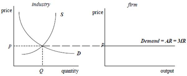
The average revenue (AR) is the price charged per unit so the average revenue curve is the demand curve. Since the price charged is fixed then the marginal revenue earned by selling an additional unit is just the price received for that unit
Short-run Equilibrium
The diagram below shows a short-run equilibrium position for a firm in perfect competition
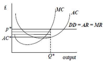
Suppose an individual firm has the following cost structure:
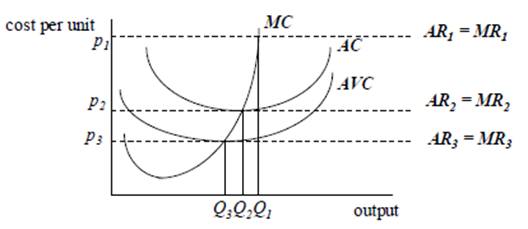
At price p1, the firm produces where MC = MR, ie Q1. At this price, the firm makes supernormal profit since price exceeds average cost.
At price p2, the firm produces where MC = MR, ie Q2. At this price, the firm makes normal profit since price is equal to average cost.
At price p3, the firm produces where MC = MR, ie Q3. At any price between p2 and p3, the firm makes less than normal profit, but it carries on in the short run because price exceeds AVC.
At prices below p3, the firm will supply nothing, since the price does not even cover its average variable cost.
Thus, the MC curve above minimum AVC is the firm's short-run supply curve. At prices below minimum AVC, the firm will supply nothing.
All firms have such supply curves.
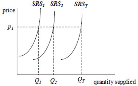
At price p1 Firm 1 supplies Q1 and Firm 2 supplies Q2, so in total they supply QT. In this way the quantities supplied at all prices can be found. The short-run supply curve for the perfectly competitive industry is the horizontal summation of the short-run supply curves of the individual firms.
Long-run Equilibrium
In the long run all factors are variable. Since there are no barriers to entry or exit, firms can enter the industry or they can leave.
If supernormal profits were being earned in the short run, then new firms (with cost curves such that they could make at least normal profit) would be tempted to enter the industry in the long run. The output of the new firms would increase the total industry supply and hence reduce the market price and the level of profit. The process would continue as long as supernormal profits were being earned.
The following diagram shows the long-run equilibrium position for the perfectly competitive firm.
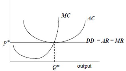
The shape of the long-run industry supply curve will reflect the way that the costs experienced by firms change as total output changes.
If increased output does not increase factor costs, then additional new firms will be attracted to the industry and the long-run supply curve will be horizontal. If the additional demand for factors of production pushes up their cost, then the long-run supply curve will slope upwards, reflecting additional output from existing firms and also, possibly, new entrants.
However, the long-run supply curve may even be downward sloping. This would occur if the additional demand allowed firms to operate in a more efficient manner (including reduced costs for factors of production that could be supplied more efficiently).
A horizontal long-run supply curve will occur in constant cost conditions.
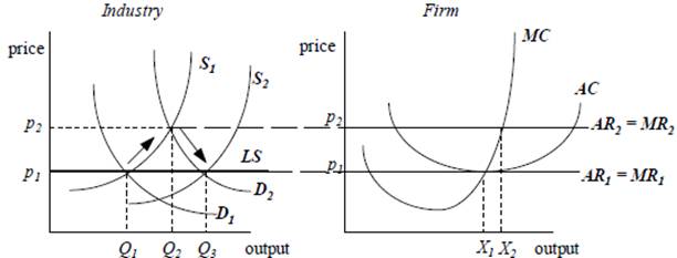
Initially, firms produce a quantity of X1 and earn normal profit. Demand for the product increases from D1 to D2, causing the price to rise from p1 to p2. As a result, firms produce X2 and earn supernormal profit.
This attracts more firms into the industry in the long run. The industry’s short-run supply curve shifts to the right, bringing down prices and profit. Since all firms are equally efficient, this process must continue until all supernormal profit is competed away. This occurs when the price has fallen back down to p1 and all firms are earning normal profit only. The original firms reduce output from X2 back to X1 in response to the lower price level.
So, what is the change in supply in the long run? Initially the industry produces Q1 at price p1. After a series of changes, the industry produces Q3 at price p1. Thus, in the long run, the price is constant (at price p1), so the long-run supply curve (LS) is perfectly elastic (horizontal) at minimum average cost.
An upward-sloping long-run supply curve will occur in increasing cost conditions. In the short run, prices will rise and firms in the industry will make supernormal profits. This attracts more firms into the industry in the long run. Firms will continue to enter the industry as long as they can make (at least) normal profit.
- If new firms face higher costs (the first condition), then firms will stop entering the industry at some stage before the price has fallen back to the original price. In this case, there will be an upward-sloping long-run supply curve, i.e. a higher price is required to increase the supply.
- If the process of expanding the industry causes such an increase in demand for a factor of production that the price of the factor of production increases (the second condition, sometimes known as the “factor price effect”), then there will be an increase in the firms’ costs and the break-even price will rise.
Therefore if either of the conditions holds, then firms will experience increasing cost conditions and the long-run supply curve will be upward sloping.
A downward-sloping long-run supply curve will occur in decreasing cost conditions. The expansion of the industry sometimes enables the industry as a whole to operate more efficiently. As the size of the industry grows, there may be an incentive for firms to set up in support of the industry. For example, specialist suppliers might evolve from the growth of the mobile phone industry, banks might establish specialist departments for dealing with the industry and training schools might be established to train workers in the specific skills required by the industry.
All these developments make it easier and cheaper for new firms to produce mobile phones. New firms are therefore willing to join the industry at successively lower prices. Thus the long-run supply curve is downward sloping.
The social optimum and perfect competition
Unlike the other market forms, the price charged to customers is equal to marginal cost in perfect competition. Therefore, unlike the imperfectly competitive market forms, perfect competition produces the socially optimal output level. There is no welfare loss under perfect competition.
If we move up from the firm to the industry, we can say that the social optimum is found in perfect competition where supply is equal to demand.
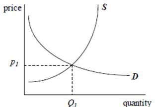
The total welfare gain from producing output Q1 is found by adding the welfare gain from each item produced, i.e. the area between the demand and supply curves up to output Q1.
Consumers’ and producers’ surplus
Another way of analysing welfare is to use the concepts of consumers’ and producers’ surplus. Consumers’ surplus is the surplus satisfaction received over that which is paid for.
Let us examine the demand curve in the following diagram.
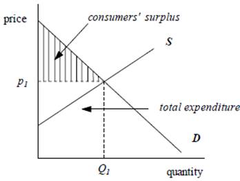
We shall assume that the price the consumer is prepared to pay for an additional unit reflects the marginal utility the consumer will obtain from the additional unit. We know that consumers need a drop in the price to encourage them to buy more of the product. This is because the marginal utility falls with increased consumption. Thus the area under the demand curve up to output Q1 shows the total value to the consumers of consuming Q1 of the product.
Since the consumers have to pay p1 for the product, the total amount spent on the product is p1 × Q1. Thus the consumer surplus is represented by the shaded area in the diagram.
The producers’ surplus is the surplus revenue received over that which is necessary to ensure supply.
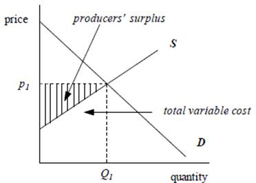
The supply curve shows the quantities that the producer is willing and able to supply at various prices. We know that the supply curve is derived from the marginal cost curve, which shows the addition to total cost as a result of producing an additional unit of output. These additional costs are additional variable costs. Thus the area under the supply curve shows the total variable cost of producing the product. This is the amount necessary to ensure supply since, in the short run; the firm will produce if the revenue exceeds the total variable cost of production.
Since the total revenue received is p1 × Q1, the producers’ surplus is therefore represented by the shaded area. The total welfare gain from producing Q1 is therefore equal to the consumers’ surplus plus the producers’ surplus, i.e. the area between the demand and supply curves up to Q1.
Monopoly
A monopoly is a firm which is the sole supplier of a good and which faces no potential rivals. To be in this position, there must be some barriers which prevent other firms entering the industry. For example, a country with a publicly-owned telecommunications company may outlaw the setting up of rival firms.
Since there is only one supplier, the demand curve that an individual firm faces is the market demand curve.Since in monopoly the firm has no rivals, the demand curve for the product is likely to be relatively inelastic.
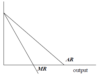
If the demand (average revenue) curve is a downward-sloping straight line, then we know that the marginal revenue curve is also downward sloping but it is twice as steep as the average revenue curve
A monopolist could make supernormal profit (AR > AC), normal profit (AR = AC) or losses (AR < AC) in the short run. (Remember, the monopolist will close down in the short run if AR < AVC.) We will draw the diagram for the monopolist making supernormal profit.
We need to draw in an average cost curve (AC) so that the difference between the demand curve (i.e. average revenue) and average cost curve at the chosen output level, Q*, illustrates supernormal profit. Remember that the average cost curve is assumed to include the opportunity cost of the owner’s time and money.
Therefore, we simply need to illustrate positive economic profits.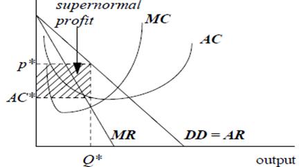
In this case, price exceeds average cost and the firm is making supernormal profit per unit of p* − AC*. Total supernormal profit is (p* − AC*) × Q*.
A monopoly does not face any competition and thus there is nothing to stop it making supernormal profit.
If a monopolist is making supernormal profit in the short run, then in the long run, new firms will be attracted to the industry. However, they will not be allowed to enter the industry and thus the monopolist is shielded from competition. The monopolist is therefore able to make supernormal profit in the long run.
The key feature of a monopoly is that it is able to make supernormal profit in the long run, as well as the short run, without worrying about competitors.
Note that some monopolies are state-owned and that state firms may not be run for the purpose of maximising profits. The analysis above would therefore not be appropriate because the chosen output level would be set by some other criteria than equating MC with MR. For example, some of the UK’s old nationalised industries were required to produce the break-even level of output, i.e. set price equal to average cost, and some were required to produce the socially optimal output, i.e. set price equal to marginal cost.
There is a strong economic argument that says that monopolies are bad for society. The principal reason for this is that under monopoly the output level is too low to maximise social welfare.
The way to see that output is too low is to look at the monopoly’s chosen output level and weigh up the costs and benefits to society of increasing output by one unit. The main cost to society will be whatever it costs the monopolist to produce the one extra unit. If there are no other costs imposed on society then the monopolist’s marginal cost is the marginal cost to society.
The demand curve shows how much consumers are willing to pay for the extra unit. Assuming that price reflects utility, the extra unit is “worth” the amount shown by the demand curve to the consumer who buys it. Assuming further that there are no external benefits, and then price can be assumed to reflect the marginal social benefit of the extra unit.
We can take the demand curve as showing the marginal benefit to society of each extra unit produced. So long as the demand curve (i.e. consumers’ valuation of each extra unit of output) exceeds the monopolist’s marginal cost curve (ie the marginal cost to society), social welfare can be increased by setting output at a higher level. The socially optimal output level is thus where the marginal cost curve cuts the demand curve.
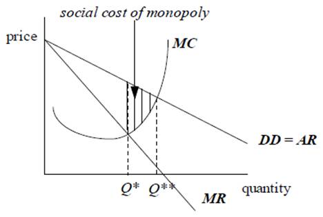
The profit-maximising output under monopoly is Q*, but the socially optimal output level is Q**. So output under a monopoly is too low for social welfare maximisation. The reduction in social welfare is shown as the shaded area. It is called the “social cost” or “dead-weight burden” of monopoly. It is found by integrating the distance between the demand curve and the marginal cost curve over the range Q* to Q**.
Monopolies restrict output, charging a price that lies above marginal cost. If we interpret the demand curve as society’s marginal benefit schedule, and the marginal cost curve as reflecting society’s marginal costs, we can show that there is a social welfare loss imposed by a profit-maximising monopoly.
The welfare loss is represented by the shaded area and results from output being too low. There may be an additional loss if we are prepared to make a value judgement about the effect of a monopoly’s pricing policy on social welfare.
Price Discrimination
Because monopolies do not face any competition (actual or potential) they may be able to charge different prices to different groups of customers.
Price discrimination exists where a monopoly firm charges different prices to different sections of the market.
If it is possible for a firm to employ price discrimination, it will be profitable to do so. The monopoly will be able to expand its output and increase its profits.
Price discrimination can operate because different customers have different demand elasticities. For example, suppose an airline has a monopoly on routes between London and Paris. Business customers have a very inelastic demand whereas tourists have a very elastic demand. If the company charges a single price, this might be too high for many tourists, who decide to go on holiday to Rome instead; whereas additional revenue could be raised from the business customers. The company would increase its revenue if it decreased the price to tourists and increased the price to commuters.
Monopolistic competition
In monopolistic competition:
- There are many firms supplying in the market.
- Each firm has a small enough share of the market that it can change its actions without influencing the behaviour of other firms.
- There is free entry and exit of firms into the industry.
- Each firm sells a differentiated product and faces a downward-sloping demand curve.
By free entry we mean that there are no barriers to entry. We assume that companies that are not currently in the industry could choose to enter the industry without set-up costs and that they would not be at a huge cost-disadvantage to the existing suppliers. By free exit we mean that, in the long run, a firm can pull out of an industry and would then save the full amount of ongoing fixed and variable costs. In other words there are no exit costs, such as decommissioning plant.
Unlike oligopoly, each firm is small relative to the market, so that if a single firm doubles its output, the other firms will hardly notice. The other firms won’t react to the actions of a single firm as they would in an oligopoly. Therefore kinked demand curve theories and strategic behaviour are not relevant for monopolistic competition. In addition, the free entry assumption rules out the possibility of cartels being successful. We can go back to considering each firm more or less in isolation.
Monopolistic competition is similar to perfect competition in that there are many small firms in the market and there is freedom of entry and exit. The main difference is that the firms in perfect competition are selling exactly the same product whereas firms in monopolistic competition are all selling something slightly different.
We know that firms in perfect competition are price takers. If a firm increases its price it would lose all its customers. But a firm in monopolistic competition has some market power: it can increase its price and not lose all its customers because it is producing something slightly different from the products produced by its competitors. There is some loyalty to the firm’s product. Firms retain some power to influence the price at which they sell. This may be due to brand loyalty and an element of product differentiation. If a corner grocer puts up his prices by 10% he will lose some, but not all, of his sales as some customers switch to alternative shops
Short-run equilibrium position for the firm in Monopolistic Competition
Each firm faces a downward-sloping demand (AR) curve that represents a small fraction of the overall market demand. This is drawn as a downward-sloping straight line DD in the figure below. The marginal revenue curve (MR) for the firm is then a downward-sloping straight line, starting at the same point as the demand curve but with twice the steepness. Than we have the usual marginal cost curve shape (MC). We can find the profit-maximising output by choosing the output level Q* where marginal cost equals marginal revenue. At the profit-maximising output price p* must be charged to ensure that this output level is sold. Now we have the average cost curve (AC) such that the marginal cost curve cuts through the minimum point on the average cost curve.
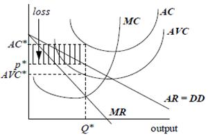
In the short run the firm in monopolistic competition could be making supernormal profit, normal profit or losses. The diagram below shows the firm making losses. The average cost curve and the average variable cost curve have been drawn so that price exceeds average variable cost but is less than average cost at Q*. AC* is the average cost of making Q*. In this case the firm is making a loss per unit of AC* − p* and a total loss of (AC* − p*) × Q*.
If the firm is making supernormal profit, the short-run equilibrium diagram is the same as for a monopolist.Long-run equilibrium position for the firm in Monopolistic Competition
The distinction between monopoly and monopolistic competition results from the assumption that there is free entry into a monopolistically competitive industry. If firms in the industry were making supernormal profits, other firms would enter the industry. The entry of new firms would increase competition in the industry and so reduce prices and profits. New firms would continue to enter the industry until all supernormal profits were “competed away”, i.e. until firms were making only normal profits.
Similarly, if firms in the industry were making negative economic profits, firms would begin to leave the industry. This follows from the assumption that exiting the industry is costless, and thus a better alternative than making negative profits. As firms left the industry, competition would be reduced and profits for the remaining firms would increase until normal profits were again made.
So the long-run equilibrium (the position from which there is no tendency to change) occurs when firms are making only normal profits.
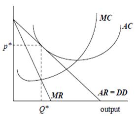
This means that an average cost curve (AC) needs to be drawn so that at the chosen output level Q*, average cost is tangential to average revenue. For this reason some economists refer to the monopolistically competitive firm’s long-run equilibrium as “the tangency equilibrium”.
Oligopoly, Duopoly
Oligopoly describes a market in which there is a small number of competing firms, each of which believes that its own actions will lead to some form of non-negligible reaction from the other firms. The more firms there are in a market, the more likely it is that the reactions of other firms will be negligible. It is difficult to determine precisely how many firms it would take to make reactions negligible. The threshold number of firms in an industry at which interactive effects can be ignored probably varies from industry to industry. So it is not possible to say exactly how many “a small number” of firms are. Industries with between, say, two and ten firms will usually be an oligopoly.
For the industry to be restricted to only a few firms, there need to be some barriers to entry, as was the case with monopoly. We discuss barriers to entry after drawing the diagram for oligopoly.
The shapes of the revenue curves depend on the power that the firm has in the market. The demand curve for a firm in perfect competition is perfectly elastic because it has no power to increase its price. If it increased its price, there would be an infinite fall in quantity demanded. To what extent can the firm in oligopoly increase its price? What will be the effect of an increase or a decrease in its price? This depends on the assumptions we make about the way in which other firms in the industry react. There are many theories about this but we are going to consider the kinked demand curve theory.
The diagram shown below for an oligopoly must be considered in two separate sections. In each case we start from the current price and quantity (ie point p*Q* which is labelled as D* in Figure 5). We first look at the D*D′ section of the demand curve that lies to the right of D*. We then look at the DD* section of the demand curve that lies to the left of D*.
An oligopolist believes that the other firms will react to changes in its output and pricing decisions. If a firm reduces prices below the current equilibrium price p*, the other firms may also cut their prices to the same extent. In this case the original firm’s market share is likely to remain unchanged. Sales will expand slightly as lower prices increase demand in the whole industry. So below the current equilibrium price the firm’s demand curve (DD′) will slope downwards with a similar elasticity to the demand curve for the whole industry.
If the firm sets a price above its current equilibrium price, there is a danger that competitors will not follow suit (in an attempt to increase their market share). The firm that increases its price will lose a lot of sales as customers switch to competing firms and its market share tumbles. So, above the current equilibrium price the firm’s demand curve (DD*) will be very flat – ie more elastic than the demand curve for the whole industry.
In this view of oligopoly, we are assuming that the other firms react in the way which is most harmful to the firm we are looking at. This is only one view of oligopoly. Some alternative views of oligopoly are discussed later.
Because the demand curve is kinked, the marginal revenue curve (MR) for the firm needs to be considered in two separate sections. You can draw in the correct marginal revenue curve for each section by pretending that the two sections of the demand curve are part of two different straight-line demand curves. The result should be a curve that is discontinuous at the current output level Q*.
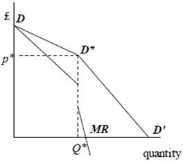
So, remembering the relationship between a straight-line demand curve and the associated marginal revenue curve, the left section of the marginal revenue curve must start at D and be twice as steep as DD*. The right section of the marginal revenue curve is twice as steep as D*D′, and is the continuation of a line starting at the same point on the price axis that a continuation of the line D*D′ would start at.
Also, the left section of the marginal revenue curve would (if continued) cut the quantity axis half way to the point where a continuation of DD* would cut the quantity axis. The right section of the marginal revenue curve cuts the quantity axis half way towards D′.
Short-run equilibrium position for the Oligopolist
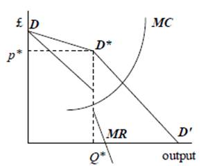
Consider the kinked demand (AR) curve DD*D′ in the figure below. We have the discontinuous marginal revenue curve (MR) and the usual marginal cost curve shape (MC) which passes through the disjointed part of the marginal revenue curve. The profit-maximisation output is thus at Q*. (If in stage 3 we had not drawn the marginal cost curve through the disjointed part of the marginal revenue curve, p* would not be the equilibrium price. We would then have been wrong to consider D* as the starting point for stage 1.).
The oligopolist's price is p*, i.e. where the demand curve is kinked. We then usually draw the average cost curve so that the marginal cost curve cuts through the minimum point on the average cost curve. In the short run we can choose to show supernormal profit, normal profit or losses. The traditional diagram of oligopoly tends to omit the average cost curve because the diagram already illustrates the key features of oligopoly.
Long-run equilibrium position for the Oligopolist
In oligopoly, it is assumed that there are some barriers to entry preventing too many firms competing in the industry. Therefore oligopolists, like monopolies, can usually make supernormal profits.
The key feature of oligopoly is that a firm must consider the reaction of other firms to its own actions. As a result, the kinked demand curve theory predicts that price and output levels may be relatively stable in an oligopolistic market.
Collusion
Since there are only a few firms under oligopoly, it would be possible for them to collude.
Collusion is where two (or more) firms jointly set their prices or outputs, divide the market among them, or make other business decisions jointly.
For example, they could agree that they would all increase their prices together above the current price. This means that they would not need to worry about the impact of a price rise on their individual market share.
Collusion implies that firms avoid competing with one another. Such activities are, typically, aimed at increasing profits above the equilibrium level and are therefore sources of inefficiency. Together the firms act as a monopolist and collusion enables them to maximise their joint profit. Collusion may take the form of the creation of trusts or cartels which are formal agreement between firms. In many countries cartels are illegal. Even where explicit collusion is outlawed, “tacit” collusion may occur.
However, there is a problem for the oligopolists. As far as the oligopolists are concerned, the problem with cartels is that they are subject to cheating. Having persuaded the other firms to restrict their output and drive up the market price, it is in an individual firm’s short-term interest to produce a lot of output to make as much profit as possible. So, there is a dilemma for oligopolists. If they all abide by the implicit or explicit arrangement to collude, they maximise joint profit. If they all cheat in the hope of increasing Brand Management Tutors and profit at the expense of rivals, joint profits will be low. Such issues are explored in the study of game theory.
Game theory
Game theory analyses the way that two (or more) players choose actions (or strategies) that jointly affect each participant.
For example, price cutting (to boost sales and profits) by one firm in an imperfect market may well be met by other firms responding with similar cuts, thereby just “ratcheting down” profits overall. Consideration of how others will react to your actions forms the basis of game theory.
Simple strategies (such as the interaction between two firms) can be analysed by way of a payoff table. This aims to map the outcomes generated by each pair of strategic choices by the firms. The essence of game theory is that a firm should select its preferred strategy assuming that the opponent is also analysing the chosen strategy and acting in its own best interests.
In some instances, analysis may reveal a dominant strategy, where one player has a best strategy no matter what strategy the other player follows. When all players have a dominant strategy, the outcome is a dominant equilibrium.
Often games have one strategy combination that is the joint optimum for the players. However, it then pays each player to switch strategy, but if both do so, each will be worse off. A particular example of this is the prisoner’s dilemma.
Consider two known criminals X and Y who have been found together with a stash of diamonds. The two are taken to the police station and questioned separately. Each knows that he will certainly be convicted of handling stolen goods. He also knows that he cannot be convicted for theft unless one of them confesses. Each of them is then offered a deal: if you confess to the theft, and your partner does not, you will be released without charge, and your partner convicted of theft. If you both confess, you will both be convicted of theft but with a lesser sentence.
The outcomes can be summarised as: no charge, handling, theft with mitigation, theft. Let us assign the following “feel good” points to each of these as: 100, –10, –100, –200. Then the payoff table is set out below. The first payoff in each bracket refers to Criminal X and the second to Criminal Y.
| Criminal Y | |||
| Strategy | Say nothing | Confess | |
| Criminal X | Say nothing | (−10, −10) | (−200, 100) |
| Confess | (100, −200) | (−100, −100) | |
So, if X confesses and Y says nothing, they will receive payoffs of +100 and −200 respectively. Looking at the sum of the payoffs, this is largest when neither confesses. However, looking at each scenario individually, it pays each criminal to confess.
Consider Prisoner X's situation: if Y confesses, then it is better if X confesses too and earns −100 rather than −200; if Y says nothing, then it is also better for X to confess and earn 100 points rather than −10. Confessing is Prisoner X’s dominant strategy since it is preferred by X regardless of what Y does. Prisoner Y faces the same situation and thus Prisoner Y confesses too. Thus the dominant equilibrium is that both confess.
The paradox is that the best option is for both prisoners to confess and earn −100 points, when it could have been −10 if they had both remained silent.
This non-cooperative game shows how independent decision making can lead to inferior results for the players. If the prisoners had colluded, they would have remained silent and received a lighter sentence.
Now let us consider two firms X and Y, each of whom can choose a high- or low-output strategy. We begin by mapping the resulting profits to (X, Y) in a payoff table:
| Firm Y | |||
| Output Strategy | Say nothing | Confess | |
| Firm X | High | (15, 15) | (45, 0) |
| Low | (0, 45) | (30, 30) | |
From the table, we can see that if Firm Y were to choose a high-output strategy, Firm X would do best by also going for high output. On the other hand, if Firm Y chooses low output, Firm X should still aim for high output. Thus for Firm X, high output is the dominant strategy. Similarly, for Firm Y the high-output strategy dominates.
However, the table also shows that, if both firms choose low output, then each will benefit (compared to both choosing high output). This demonstrates the benefit of collusion.
Game theory can be used to develop important principles of microeconomics. In particular, it can be shown that, in a perfectly competitive environment, non-cooperative behaviour of many independent firms produces an efficient allocation of resources. Co-operation and collusion lead to economic losses to consumers. This suggests why governments want to enforce anti-trust laws that contain harsh penalties for those who collude to fix prices or divide up the markets.
Note, however, that the presence of externalities – results of activities which impose costs (or benefits) on others outside the market place, which are not fully reflected in market prices – may make the non-cooperative equilibrium inefficient. This may then provide a justification for government intervention.
Microeconomics Assignment Help | Microeconomics Help | Form of Markets | Competition and Market Structures | Competitive Market | Market Structures | Market Forms | Online tutoring


