Microeconomics Costs Assignment Help
Costs
Cost of production
A firm uses scarce resources (land, labour and capital) to produce its products. In doing so, it has to pay something to the owners of these factors of production. For example:
- Rent to be able to use a building
- Wages to employ workers
- Raw material costs. The quantity of raw materials actually used, rather than the amount purchased, is the relevant economic concept.
- Interest payments to people who lend money to the firm.
- Depreciation cost of a machine. This measures the reduction in the value of a machine over a year. It is a better way of assessing the cost of capital equipment than the amount spent purchasing new machines.
Microeconomics Costs Assignment Help By Online Tutoring and Guided Sessions at AssignmentHelp.Net

While the above explained costs are explicit cost, there are few implicit costs too, that are considered by economists in the total cost of production. These implicit costs are as follows;
- The opportunity cost of the money that the owner has tied up in the business. This is the reward or return that the owner could have earned on his money in its next best alternative use. For example, the money could have been used to buy shares, bonds or property.
- The opportunity cost of the owner's time. The owner could spend time earning money elsewhere. This lost money is also an “economic cost”. (There may be non-monetary aspects to running one's own business that compensate for this item, such as a feeling of satisfaction and achievement. These should be included as a negative cost.)
Explicit costs – explicit costs have measurable cash flows, the costs relate to payment for resources. Examples are wages, rent, and raw material costs.
Implicit costs – these are opportunity costs of using the firm's resources; they are often not included in the accounting statements. Examples are wages or rental, which are not claimed by the owner of the business.
Kinds of costs
Fixed costs and Variable Costs
- Variable costs: these are costs that rise as output increases, the average variable cost is the total variable cost divided by the number of units produced.
- Fixed costs: these costs do not vary with the level of output. The average fixed costs are the total fixed cost divided by the number of units produced; it will decline as production increase.
Total, Marginal and Average Costs
- Total cost: this is the cost of production. It is the sum of both fixed costs and variable costs.
- Marginal costs: increase in total costs caused by an increase in output of one unit.
Marginal cost (MC) = d(total economic cost)/ d(output)
- Average cost: defined as total costs divided by the output level. This is cost per unit of output.
AC = ![]()
Short Run Marginal Cost Curve
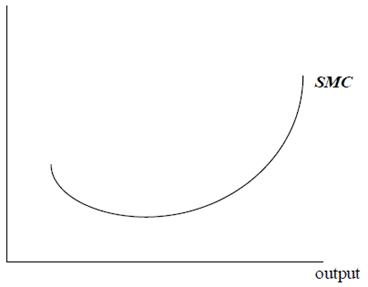
In the short run, the firm can only increase output by increasing the use of its variable factor, usually taken to be labour. Thus, assuming the cost of labour is constant; the marginal and average cost will depend on the productivity of labour. If we assume that labour is the only variable input, there is a direct inverse relationship between the marginal productivity of labour and short-run marginal costs. Each worker costs the same to employ. If marginal productivity decreases, each additional worker is adding less than the worker before. It takes successively more workers to make each extra unit of output. As productivity falls, marginal costs increase. Since the marginal product of labour is likely to rise and then fall, the short-run marginal cost of production is likely to fall and then rise. The short-run marginal cost (SMC) curve illustrated in the figure below is typical of many manufacturing industries.

Relationship between Average Cost, Average Fixed Costs, Average Variable Costs and Marginal Costs
The table below shows the total cost, average cost and marginal cost of producing from zero to 10 units of output.
| Output | Total Cost | Average Cost | Marginal cost |
| 0 | 10.00 | ||
| 1 | 11.00 | 11.00 | 1.00 |
| 2 | 11.51 | 5.75 | 0.51 |
| 3 | 12.41 | 4.14 | 0.90 |
| 4 | 14.00 | 3.50 | 1.59 |
| 5 | 16.46 | 3.29 | 2.46 |
| 6 | 19.91 | 3.32 | 3.45 |
| 7 | 24.44 | 3.49 | 4.53 |
| 8 | 30.12 | 3.77 | 5.68 |
| 9 | 37.00 | 4.11 | 6.88 |
| 10 | 45.13 | 4.51 | 8.13 |
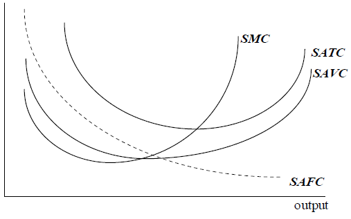
The table shows the expected pattern of marginal cost. At low levels of output, marginal cost falls as output increases. As output continues to rise, marginal cost starts to increase. The rate of increase accelerates as output continues to rise. The table also shows that the average cost curve is U-shaped. As output increases from 1 unit to 5 units, the average cost falls from 11 to 3.29. As output increases beyond 5 units, the average cost increases. If we divide short-run total costs by the number of units of output, we obtain short-run average total costs. Similarly Short-run average fixed costs = short-run fixed costs / output Short-run average variable costs = short-run variable costs/ output Figure below shows short-run average total costs (SATC), short-run average fixed costs (SAFC) and short-run average variable costs (SAVC). These are found by dividing the cost curves in Figure 4 by the level of output. It also shows short-run marginal costs (SMC).

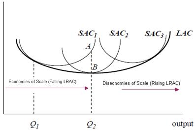
As can be seen in the above figure the marginal cost curve cuts through the minimum points of both the average cost curve and the average variable cost curve. This relationship can be explained as follows. If the marginal cost is less than the average cost, then the addition to total cost of producing an additional unit of output is less than the average cost so the average cost must fall. In above Table, the marginal cost of producing the second unit is only $0.51 when the average cost of producing the first unit was $11. By producing the second unit, the average cost falls to $5.75. If the marginal cost of producing an additional unit of output is equal to the average cost, then the average cost is unchanged. If the marginal cost of producing an additional unit of output is more than the average cost, then the average cost must rise. Whilst SAFC continuously decline as output expands, SMC initially decline but at a certain output level they start to increase pushing up the SAVC and SATC. If a firm has the flexibility to alter its plant size then the long run average total cost curve becomes a combination of the short-run average total cost curves. In the long run, the firm can increase output by increasing the use of all of its factors of production. In other words, the firm can change the whole scale of its operation. Thus, the marginal and average cost will depend on the returns to scale. The long-run average cost is likely to fall initially as output increases because of Brand Management Tutors (or increasing returns to scale). Firms might find that within a certain range of output, long-run average cost is constant. This is termed constant returns to scale. However, as output continues to increase, the long-run average cost is likely to rise because of diseconomies of scale (or decreasing returns to scale). In the long-run, the quantities of all input factors can be varied, in particular, the level of capital can be varied. LAC is the long-run average cost when it has been possible to re-optimise the amount of capital available and labour used. In the short-run, the level of capital is fixed. Each short-run average cost curve shows the average cost for a different level of capital. (Therefore moving along a short-run average cost curve represents a change in the level of the variable factor of production, labour.) Suppose a company wishes to produce an output level of Q1. Call the optimal (long-run) level of capital needed to produce this level K1. SAC1 is the short-run average cost when the level of capital is K1. Moving away from Q1 in either direction, short-run average costs are above long-run average costs. The optimal amount of capital needed to produce less than Q1 will be lower than K1. Similarly, the optimal amount of capital needed to produce more than Q1 will be more than K1. The lower costs on LAC can only be reached in the long run when it has been possible to re-optimise the amount of capital.

For example, suppose the company wants to increase output to Q2. In the short-run, it must increase the level of labour (since the level of capital is fixed). This represents a move along SAC1 to point A. In the long run, the company can re-optimise the level of capital available to K2, and so move on to SAC2 (the short-run average cost when the level of capital is K2). Average cost will fall to the point B. The relationship between the long-run average cost curve and the long-run marginal cost curve is exactly the same as the relationship between the short-run average cost curve and the short-run marginal cost, i.e. the long-run marginal cost curve cuts the long-run average cost curve at its lowest point
Microeconomics | Microeconomics Help | Costs | Microeconomics Costs| Microeconomics Cost | Short Run Variable Costs | Online tutoring


