IS LM Model

Let us consider a closed economy for which we will derive the short-run IS-LM model. Assume that in the beginning the economy has equilibrium in both the goods market and the money market. Let us describe this economy’s goods market and money market

Goods market:

The consumption function is given by C = c0 + c1(1-t) Y, where C is consumption; Y is income; t represents a proportional tax; and c0 is the consumption when income is zero and c1 is the marginal propensity to consume. Both c0 and c1 are positive constants.

The Investment function is given by: I = b0 – b1i, where I is investment; i is the interest rate; and b0 and b1 are positive constants. b1 is known as the interest rate sensitivity of Investment spending

The government spending is a positive constant denoted as G = G, where G is a positive constant
Let us combine the goods market equations to derive an expression for Y as a function of i. This will be called the IS curve).

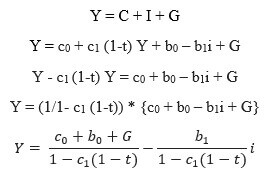
IS relation shows an inverse relationship between interest rate and output(income) for which goods market is in equilibrium.

Money market:

The money demand function is estimated to be M_d = P (m₀ + m₁Y – m₂i), where Md is money demand; P is the price level; m0 (a positive constant) represents exogenous changes to Md ; and m1 and m2 are also positive constants

Let Ms represent money supply which is taken to be given by the central bank.

Then the Money market equilibrium equation is

{`
Ms = Md
P (m0 + m1Y – m2i) = Ms
(m0 + m1Y – m2i) = Ms/P
Ms/P - m0 + m2i = m1Y
i = 1/m2 (m0 – Ms/P) + m1/m2 Y
`}

The LM curve is upward sloping because higher income results in higher demand for money (because of higher transactions demand for money). This results in higher interest rates so that people are induced to hold lesser money as cash and demand for money is reduced.

Let us now graph the IS curve and the LM curves on the same diagram, putting interest rate on the vertical axis and income(output) on the horizontal axis and labelling the curves as IS curve and LM curve respectively. We will also label the equilibrium interest rate and output, i0 and Y0, respectively. The equilibrium in the IS-LM model is then at a point like e1 where both the goods market and the money market is in equilibrium simultaneously.

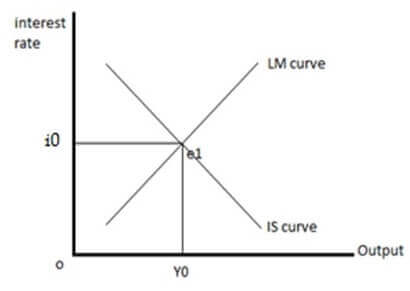
Shift of IS curve

Suppose the government increases its spending by ∆ G. Which curve will shift, if any? Calculate by how much it will shift and draw a diagram that shows the impact of this policy.

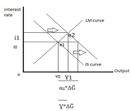
When government increases its spending, IS curve will shift to the right. At the initial interest rate i0, the money market will be in equilibrium but the goods market will no longer be in equilibrium. Due to increase in government spending, the output(income) will increase which will further lead to an increase in money demand. This will lead to an increase in interest rate as well. However, as interest rates will go high it causes decrease in investment. This phenomenon is known as crowding out. Thus, the shift in IS curve due to change in government spending will be αG*∆G̅. But the actual increase in output(income) will only be

Ɣ*∆G̅ , where Ɣ = αG / 1+b/h * k* αG
Here Ɣ is also known as the fiscal policy multiplier.

CROWDING OUT

What will happen to investment as a result of the increased government spending?

The increase in government spending will cause a multiplier increase in income(output). This will stimulate people’s transaction demand for money. To decrease the transaction demand for money, the interest rates will have to increase so that people are unwilling to hold too much money as cash. This will lead to an increase in interest rate. Increase in interest rate due to government spending will cause the investment spending to fall as interest rate and investment are inversely related. This phenomenon in which an increase in government expenditure leads to a decline in private business spending(investment) is known as crowding out. Thus, government spending has crowded out private investment spending.

Expansionary Fiscal Policy: Cutting tax rate impact on IS Curve

Suppose that the government decides to cut taxes instead of increasing spending. Analyse and explain the effects of this expansionary fiscal policy using a diagram.

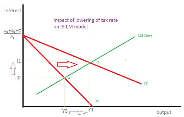
Any change in the tax rate will be reflected by change of the IS curve. Remember that the IS curve equation is

Which can also be rewritten as

Thus, the coefficient of Y is - (1-c₁ (1-t))/b₁. A decrease in t will lead to a tilt in the IS curve and IS curve will become flatter. However, the IS curve will not undergo a parallel shift as the IS curve will still intersect the vertical axis at c₀ + b₀ + G/b₁ no matter what the value of tax rate(t).

Combination of Fiscal Policy and Monetary Policy

Using the IS-LM model, let us explain what can be done to offset the changes in the interest rate caused by increased government spending and, at the same time, keep output from declining. (In other words, we will suggest a way to bring the interest rate back to the level it was at before increase in government spending took place without causing a reduction in output).

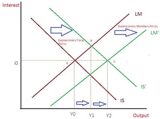
Expansionary monetary policy can be done to offset the changes brings by fiscal policy. Monetary policy will bring back the interest rate to its initial position while increasing output even more from Y1 to Y2. The from the initial equilibrium at A, we will move to equilibrium at B because of higher government spending (at which interest rate is higher and output is also higher). At the same time because of increase in money supply due to expansionary monetary policy, the LM curve will shift towards right as well. This will cause the interest rate to fall back to i0 and income to rise further from Y1 to Y2. Thus, the final equilibrium will be at a point like C.