Operations Management Assignment Answer

Production / Operations Management
Finding the Best Variables to Place in Solution for the Simplex Method of LP One last time, refer to the tableau (matrix) found in Problem #1, Supplement #4, Supplement #5 and Supplement #6 to show the initial solution for Real Deal Distributors:

Initial Solution Tableau (Matrix)

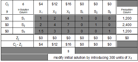
The remaining steps of the simplex method, while somewhat cumbersome when done manually, can be executed quickly and accurately with one of several readily available computer software packages.

Steps 5 and 6, selection of entering and leaving variables, can be seen on the next page in the versions of the tableau (matrix) which show different parts of the transition between the initial solution tableau and the second tableau:

Transitions Between the Initial Solution Tableau and the Second Tableau:

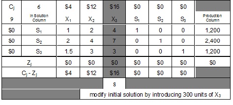
An examination of the Cj - Zj row in the initial solution tableau indicates that further improvement is possible, since there are three positive values in this row. Adding a unit of a variable linked to one of these positive values would result in a net increase in the objective function.

As shown by the shaded column above, X3 should be selected as the entering variable, since it has the highest positive value in the Cj - Zj row and, therefore, would result in the highest net increase in the objective function. If we add a unit of X3 into the solution, then the objective function is increased by $16. Or, if we add a unit of X2, the solution is improved by $12. Or, adding a unit of X1, would result in a $4 increase. Additional units of S1, S2 and S3 would have no effect on the objective function, since each has a Cj - Zj value of $0.

At each stage of the problem, we can introduce only one new variable. Each potential new variable should be evaluated so that the most attractive one can be chosen. In this case, X3 is the most advantageous variable on a per-unit basis, so it is the one that should be selected.

Why will variable S1 be chosen to leave the solution? In this problem, we can have only three variables in the solution at one time, one per constraint (restriction) equation. If a new variable is introduced, then an existing variable must leave the solution.

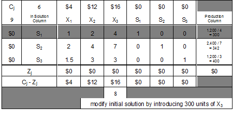
Since we wish to introduce X3 into solution, either S1, S2, or S3 must leave solution. To find the variable that should leave the solution, we must focus on the substitution rates between X3 and S1, S2 and S3 (the variables in the initial solution). Each X3 will use 4 units of S1 and there are 1,200 units of S1 available to use. Therefore, if we consider only hours of packing time (S1), then a maximum of 300 X3s can be produced, as shown in the far right column above. Further, if we consider pounds of packing material, a maximum of 2400 / 7 = 342 X3s can be brought into solution. Still further, there are enough idle minutes of inspection time (S3) to allow 400 X3s to be produced (1,200 / 3 = 400).

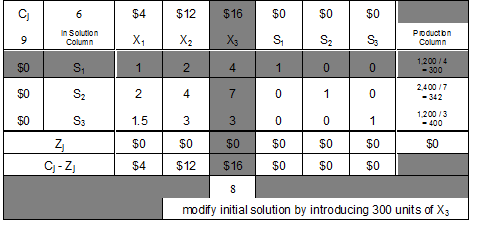
However, since all restrictions must be met simultaneously, we can see that available resources are adequate for bringing 300 units of X3 into solution. Simply stated, we must always choose the smallest result when we divide each S (or B) value by its corresponding A value.

If we bring 300 units of X3 into solution, then all hours of packing time will be used up to produce X3s. Thus, hours of packing time is the resource that keeps us from introducing more than 300 X3s (it is the limiting resource at this stage).

Note the above transition tableau which shades both the column of the variable that will be entering solution (X3) and the row of the variable that will be leaving solution (S1). The cell where this pivot column and pivot row intersect is significant as it contains the coefficient known as the pivot element. The latter (the pivot element) is an important component in the formulas that are used to revise / change / update each successive tableau (matrix) in route to the optimal / final tableau (matrix).

Returning to our Real Deal Distributors problem, after introducing the new variable X3 into solution, we must revise each row of the solution matrix to reflect the changes. These revisions / calculations can be accomplished manually using three distinct formulas one for the pivot row and two for the non-pivot rows:

Pivot row formula = Old coefficients of the pivot row / Pivot element
Pivot ratio (part of non-pivot row formula) = Old non-pivot row coefficient in the pivot column / Pivot element
Non-pivot row formula = Old non-pivot row coefficient - (Corresponding pivot row coefficient x Pivot ratio)
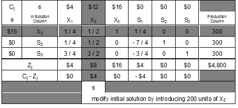
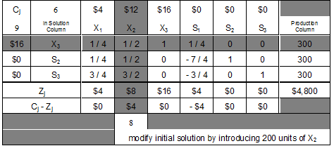
As can be seen in the following revised (second) solution tableau (matrix), the column headings are the same, but the row headings, restriction coefficients and production quantities have changed.
Revised (Second) Solution Tableau (Matrix)

In the above revised (second) solution, to bring 300 units of X3 into solution, we had to give up all 1,200 units of S1 (1,200 hours of packing time) that is, we gave up all the S1s (hours of packing time) that were formerly in solution. Further, S1 is the variable that leaves solution. It seems logical for S1 to leave since it is all committed (being used) at this point. In summary, we are producing 300 X3s and no X1s or X2s. We also still have 300 S2s (300 pounds of packing material) and 300 S3s (300 minutes of inspection time) leftover in solution (available to use). Still further, we have generated $4,800 in profit ($16 x 300 = $4,800).

For our Real Deal Distributors problem, the revisions / calculations needed to move from the initial solution tableau (matrix) to the second tableau (matrix) shown above are:

For X3 Pivot row:
Old coefficients of the pivot row / Pivot element
1 / 4 2 / 4 = 1 / 2 4 / 4 = 1 1 / 4 0 / 4 = 0 0 / 4 = 0 1,200 / 4 = 300
Pivot ratio for S2 Non-pivot row:
Old non-pivot row coefficient in the pivot column / Pivot element
7 / 4
For S2 Non-pivot row:
Old non-pivot row coefficient - (Corresponding pivot row coefficient x Pivot ratio)

2 - (1 x 7 / 4) = 8 / 4 - 7 / 4 = 1 / 4
4 - (2 x 7 / 4) = 16 / 4 - 14 / 4 = 2 / 4 = 1 / 2
7 - (4 x 7 / 4) = 7 - 7 = 0
0 - (1 x 7 / 4) = 0 - 7 / 4 = - 7 / 4
1 - (0 x 7 / 4) = 1 - 0 = 1
0 - (0 x 7 / 4) = 0 - 0 = 0
2,400 - (1,200 x 7 / 4) = 2,400 - 2,100 = 300

the S3 Non-pivot row to move from the initial solution tableau (matrix) to the second tableau (matrix)? You have the answers can you show me how to get them?

the entire procedure is repeated using this tableau (and succeeding tableaus) as the new starting point. We keep going with this process until we get to a revised solution tableau (matrix) that indicates no further improvement is possible. This point is reached when all of the values in the Cj - Zj row are either zero or negative. This means that there are no variables left to bring into solution that would increase the objective function therefore, the optimal solution has been reached.